📊 The Statistical Toolbox: Residuals, Correlation, and Determination

🏗️ The Big Three: What are they?

🔗 The Connection: How they fit together

Think of it like a puzzle:

1. Correlation ($r$) is the raw relationship between $X$ and $Y$.
2. Residuals are the pieces that don't fit the pattern.
3. Coefficient of Determination ($R^2$) is the final grade for the whole puzzle.

🚦 Usage Summary

• Use $r$ to see if there is a relationship at all.
• Use $R^2$ to see how useful your model is for the big picture.
  • $R^2$ represents the proportion of the total variation in the dependent variable ($y$) that is explained by the independent variable ($x$).
  • In other words, $r^2$ is the "Explained" part of the variation. We find it by subtracting the "Unexplained" ratio from 1
• Use Residual Patterns to see if your model is biased or broken.
• Use Standard Deviation of Residuals (${\sigma }_r$) to tell someone: "My prediction is probably off by ± [this much] in real units."

Two Ways to Calculate $R^2$: Which one and When?

There are two formulas for $R^2$. Here is the breakdown:

1. The "Shortcut" Method (using Correlation)

• When to use: When you already have the correlation coefficient ($r$).
• Meaning: It tells you that the variance explained is exactly the square of the linear strength.
• Limitation: This only works for Linear Regression with one independent variable.

2. The "Residual" Method (using Sum of Squares)

• When to use: When you have the actual data points and the regression line. This is the most powerful way because it works even for complex models (Multiple Regression).
• Meaning: It calculates: $1-(\text{Unexplained Variation}/\text{Total Variation})$.
• Analogy: If you have 100 gallons of "mystery" (Total Variation) and 15 gallons are still "mysterious" (Residuals) after your explanation, then you explained $1-15/100=85\mathrm{\%}$.

📉 Deep Dive: Residuals & Variation

1. Residual ($r_i$)

• Meaning: A residual is a measure of how well a line fits an individual data point.
  A residual is the vertical distance between an actual data point and the regression line.
• Connection: If you sum all your residuals (In Linear Regression) , they should equal zero.
  If you square them and add them up, you get the Residual Sum of Squares ($S{S}_{res}$), which represents the "unexplained" portion of your model.

• The Goal: In a perfect model, the sum of residuals is always 0.
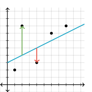• The residual for the point (4,3) is [-2]

2. Residual Sum of Squares ($S{S}_{res}$)

• Meaning: This is the Unexplained Variation. This is the variation the line couldn't explain—the distance between the points and the line.
• Connection: Lower $S{S}_{res}$ means a higher $R^2$ (a better fit!).

3. Variance of Residuals (${\mathrm{V}}_{\mathrm{r}}$)

• Meaning: The average squared error. It tells us the "spread" of our mistakes.

4. Standard Deviation of Residuals (${\sigma }_r$)

• Meaning: Frequently called the Standard Error of the Estimate.

• Why it's crucial: This is the "Typical Error." If ${\sigma }_r=2.5$, it means your predictions are usually off by about 2.5 units.
• Use: While $R^2$ gives you a percentage (relative), ${\sigma }_r$ gives you an error in the actual units (absolute), like inches or dollars.$${\sigma }_r=\sqrt{V_r}$$

5. Root Mean Square Error ($S{S}_{line}$)

Used to measure Accuracy in the same units as your data.

• Meaning: It is the standard deviation of the residuals. It tells you, on average, how far off your predictions are from the actual values.
• Connection:
  • $RMSE$ is the square root of the average squared residual.
  • While $r^2$ tells you the percentage of accuracy (e.g., 89%), RMSE tells you the magnitude of the error (e.g., "Our price prediction is off by $500 on average").
• Often used interchangeably with the standard deviation of residuals in this context

5. Total Variation ($S{S}_{total}$)

• Meaning: It is the starting baseline for all error calculations. It represents 100% of the movement we are trying to explain. It represents the total "chaos" or spread in your $y$ values relative to their average (${\mu }_y$).
• Total Variation ($S{S}_{total}$): This is the sum of squared differences from the mean ${\mu }_y$

🛠️ Working Example (Corrected)

Data points: (1,1), (2,2), (2,3), (3,6)

1: Summary Stats

i. Means (${\mu }_x,{\mu }_y$)

ii. Standard Deviations (${\sigma }_x,{\sigma }_y$)

This measures the "spread" of our data around the mean. We'll use the population formula for this high school example: $\sigma =\sqrt{\frac{\sum (x-\mu {)}^2}{n}}$.

iii: Coefficient Correlation ($r$)

The correlation $r$ tells us the strength and direction of the linear relationship. Using the formula

• Interpretation: This is a very strong positive correlation!

2: The Equation of the Regression Line ($\hat{y}=mx+b$)

• Slope ($m$): $r\cdot \frac{{\sigma }_y}{{\sigma }_x}=0.945\cdot \frac{1.871}{0.707}=\mathbf{2.5}$
• Intercept ($b$): ${\mu }_y-m({\mu }_x)=3.0-2.5(2.0)=\mathbf{-}\mathbf{2.0}$
• Line: $\boxed{{\displaystyle \hat{y}=2.5x-2.0}}$

3: Residual Breakdown Table

i. Residual/Unexplained Variation ($S{S}_{res}$)

4: Total Variation ($S{S}_{total}$)

It is the starting baseline for all error calculations. It represents 100% of the movement we are trying to explain.

• Meaning: It represents the total "chaos" or spread in your $y$ values relative to their average (${\mu }_y$).
• Total Variation ($S{S}_{total}$): This is the sum of squared differences from the mean ${\mu }_y$

5: FINAL Calculation of Coefficient of Determination

• Method 1 ($r^2$):

• Method 2 (Residuals):

Step 6: Additional Interpretations

• Variance of Residual ($V_r$): Average of squared residuals:

• Standard Deviation of Residual (${\sigma }_r$)

• Root Mean Square Error ($S{S}_{line}$)

Observations for "Correlation Coefficient" $(r)$

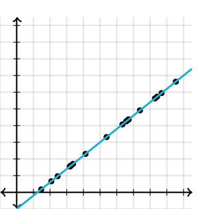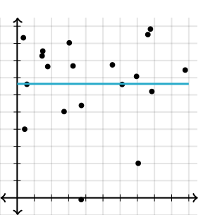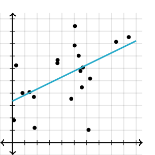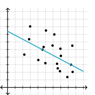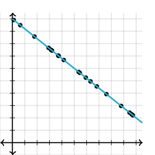[r=1], which is perfect positive correlation	[r=0], which is no correlation	[r=0.5], which is weak positive correlation	[r=-0.5], which is weak negative correlation	[r=-1], which is perfect negative correlation