Regularization

Regularization is a set of techniques that lower the complexity of a neural network model during training, and thus prevent the overfitting.. Conceptually, it forces the network to be simpler. It artificially restricts the model's flexibility so that it cannot memorize the noise, forcing it to focus only on the strongest, most generalizable patterns.

In mathematical terms, many regularization techniques work by adding a "penalty" to the loss function.

Total Loss = Data Loss + λ (Regularization Penalty)

(Where $λ$ is a number you choose to decide how harsh the penalty should be).

There are three very popular and efficient regularization techniques called L1, L2, and dropout.

I. L1 and L2 regularization

L1 and L2 regularization are techniques used in deep learning (and more broadly in machine learning) to prevent overfitting by adding a penalty to the loss function.
This penalty discourages the model from fitting the noise in the training data, thereby improving its generalization to unseen data.

L1 regularization (Lasso)

L1 regularization, also known as Lasso (Least Absolute Shrinkage and Selection Operator), adds a penalty equal to the absolute value of the magnitude of coefficients.
The modified loss function with L1 regularization looks like this:

\begin{array}{r} \underset{Loss function with no regularization}{\underset{⏟}{L o s s = E r r o r (y, \hat{y})}} \underset{Loss function with L1 regularization}{\underset{⏟}{L o s s = E r r o r (y, \hat{y}) + λ \sum_{i = 1}^{N} | w_{i} |}} \end{array}

Advantages

Sparsity: It is a harsh penalty that drives the weights of less important features down to exactly zero. This makes L1 great for "feature selection," as it completely ignores useless inputs, resulting in a sparse, lightweight model. The model hence becomes simpler, focusing only on the most important features.
Interpretability: Because some weights become zero, the resulting model can be easier to interpret.

Use Case

When you suspect that only a small number of features are actually relevant to the task.

L2 regularization (Ridge / Weight Decay)

L2 regularization, also known as Ridge regression, adds a penalty equal to the square of the magnitude of coefficients. The modified loss function with L2 regularization looks like this

\begin{array}{r} \underset{Loss function with L2 regularization}{\underset{⏟}{L o s s = E r r o r (y, \hat{y}) + λ \sum_{i = 1}^{N} w_{i}^{2}}} \end{array}

Advantages

Weight Decay: Instead of forcing weights to zero, it forces all weights to be as small as possible. L2 regularization penalizes large weights more heavily, thus prevents any single neuron from having too much influence over the final prediction.
Smoothness: Unlike L1 regularization, L2 doesn't drive the weights to exactly zero, but instead makes them smaller and more evenly distributed.

Use Case

L2 regularization is useful when you believe that most features contribute to the prediction, in varying degrees.

Differences between L1 and L2

	L1 regularization	L2 regularization
Penalty	L1 regularization adds a penalty proportional to the absolute value of the weight coefficients, leading to sparse models.	L2 regularization adds a penalty proportional to the square of the weight coefficients, leading to smaller but non-zero weights.
Feature Selection	L1 tends to produce sparse solutions, effectively selecting a subset of features	L2 tends to shrink weights uniformly
Gradient Behavior	The gradients of L1 regularization are not continuous, which can lead to convergence issues in optimization	L2 has continuous gradients, making optimization smoother.

II. Dropout Regularization

Dropout is a regularization method approximating concurrent training of many neural networks with various designs.
Dropout is the equivalent of training several independent, smaller networks on the same task. The final model is like an ensemble of smaller networks, reducing variance and providing more robust predictions.
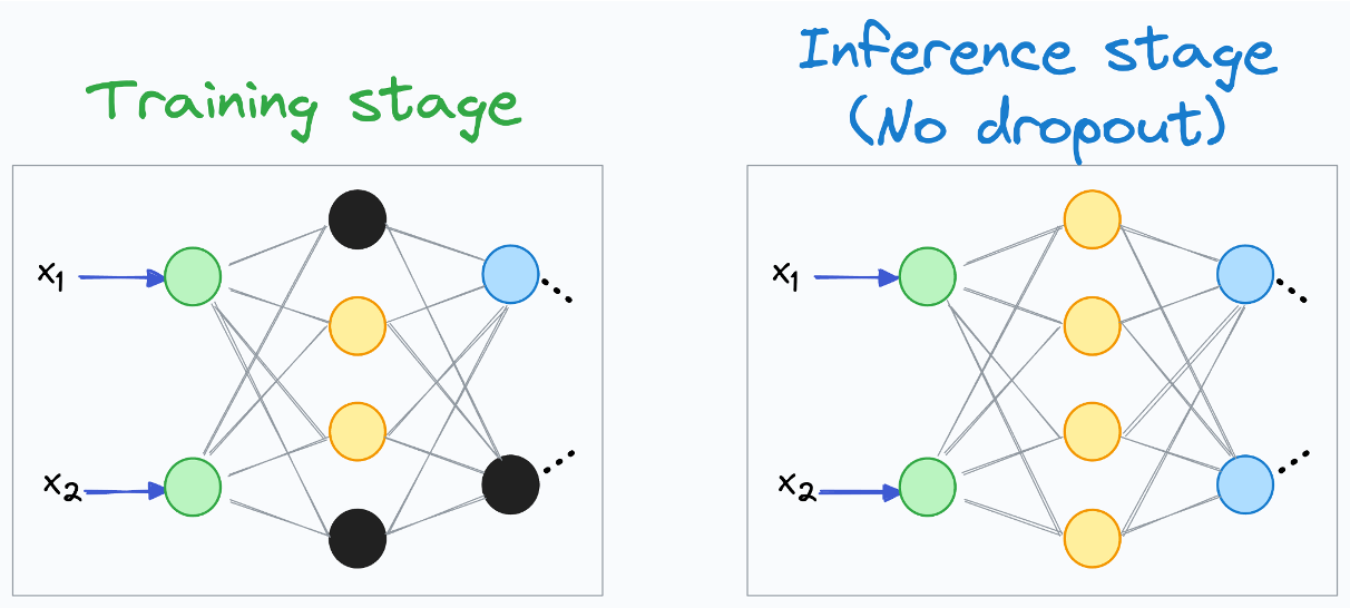
During training, dropout prevents certain neurons from participating in the forward or backward propagation process by randomly turning them “off” for each mini-batch. This ensures that the network learns from robust features and does not over-rely on particular neurons.

Process of Dropout - Training Phase

1. Define Dropout Rate ( $p$ ):

Dropout Rate is a hyperparameter — $p$ , which represents the probability of a neuron being "dropped". Common values for $p$ range from $0.2$ to $0.5$ .
Example: $p = 0.5$ means 50% of neurons will be dropped).

2. Random Deactivation:

For each mini-batch, random neurons are deactivated (set to zero) by multiplying their activations with a binary mask. This mask is a matrix of $0$ s and $1$ s drawn from a Bernoulli distribution.

\begin{array}{r} m a s k_{i} \sim Bernoulli (1 - p) \end{array} m a s k_{i} = {\begin{cases} 0 & Deactivate neuron i \\ 1 & Keep neuron i active \end{cases}

3. Dropping Neurons:

Each layer's activation is multiplied element-wise by this binary mask. If a neuron's corresponding mask value is $0$ , its activation is completely zeroed out for that specific forward pass. It effectively "disappears" from the network temporarily.

4. Forward Pass:

The modified, "thinned" network computes the predictions. Because some neurons are missing, the remaining neurons must step up and handle the workload, preventing complex co-adaptations (where neurons rely too heavily on each other).

5. Backward Pass (Backpropagation):

During the backward pass, gradients are only calculated and applied to the weights of the neurons that were active (kept) during the forward pass. The dropped neurons do not contribute to gradient computations. Gradients flow only through active neurons.

6. Repeat Per Mini-Batch:

On the very next batch of data, a brand new random mask is generated. Different neurons are dropped, and the process repeats.

7. Inverted Dropout (The Modern Standard)

In standard Dropout, dropping neurons during training reduces the expected value of the layer's overall output. To compensate for this, modern deep learning frameworks use a variation called Inverted Dropout
- In Inverted Dropout, the activations of the kept neurons are scaled up during training by a factor of $\frac{1}{1 - p}$ .
- If you keep $80 %$ of the neurons ( $p = 0.2$ ), the remaining neurons' outputs are multiplied by $\frac{1}{0.8} = 1.25$ .
This mathematical trick ensures that the expected value of the layer's output remains consistent across both training and testing, shifting the computational burden entirely to the training phase.

Testing Phase

During testing, dropout is not applied, as the intention is to evaluate the entire network without randomness. Instead, the weights learned during training are scaled to account for the earlier dropout.

1. Disable Dropout:

All neurons remain active during the inference process. The dropout masks used during training are no longer applied.

2. Scale Weights for Each Layer:

The weights for each layer are scaled down by 1−p1 - p1−p, compensating for the dropout used during training: $w_{i}^{scaled} = w_{i} \cdot (1 - p)$
This scaling ensures that the contribution of each neuron matches what was learned during training.

3. Forward Pass:

Compute activations for all neurons without randomness or adjustment from dropout masks.

4. Final Prediction:

The model combines activations from all neurons to generate predictions. The scaling ensures stable performance by averaging over the potential participation of neurons during training.

III. Regularization by Early Stopping

In Regularization by Early Stopping, we stop training the model when the performance of the model on the validation set is getting worse-increasing loss or decreasing accuracy or poorer values of the scoring metric.
By plotting the error on the training dataset and the validation dataset together, both the errors decrease with a number of iterations until the point where the model starts to overfit. After this point, the training error still decreases but the validation error increases.
So, even if training is continued after this point, early stopping essentially returns the set of parameters that were used at this point and so is equivalent to stopping training at that point.
So, the final parameters returned will enable the model to have low variance and better generalization.

Advantages

Reduces risk of overfitting.
No additional cost

test