Convolutional Neural Networks (CNNs)
1. What is Convolution operation?
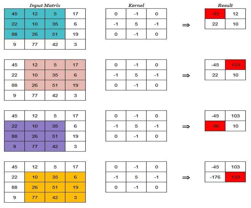
This layer is the first layer that is used to extract the various features from the input images. It involves sliding a small matrix (called a kernel or filter) over the image and performing mathematical calculations (weighted sum) at each step to create a new, transformed representation called a feature map.
Why Use Convolutions?
Before CNNs, standard neural networks flattened images into 1D arrays immediately, which destroyed the spatial relationships between pixels. Convolutions solve this problem while providing several key advantages.
- Weight Sharing: Instead of learning a separate weight for every single pixel in an image, a convolutional layer learns one small filter (e.g., 9 weights for a 3x3 filter) and applies it uniformly across the entire image. This drastically reduces the number of parameters and computational cos
- Local Connectivity: The operation only evaluates small, localized patches of the image at a time. This allows the network to understand local patterns, such as how a specific cluster of pixels forms a curve, an edge, or a corner.
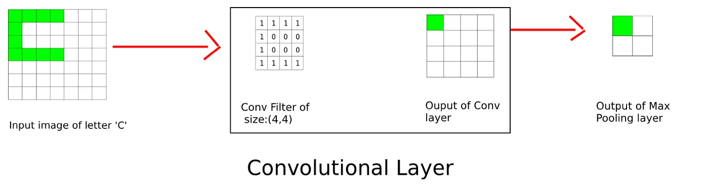
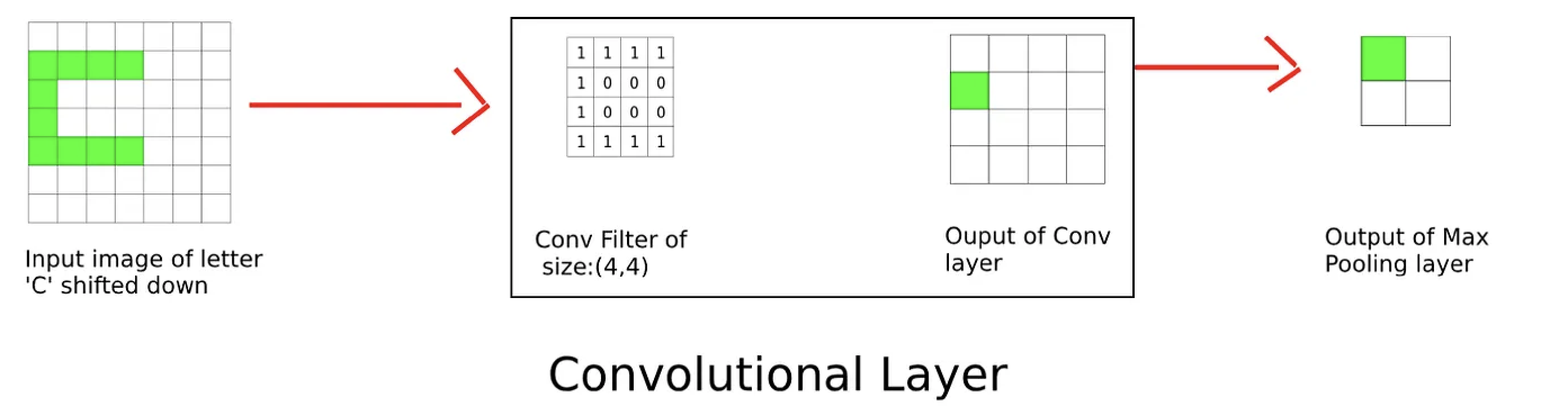
- Translation Invariance: Because the same filter slides across the whole image, it can detect a feature no matter where it is located. If a specific texture appears in the top-left corner of one image and the bottom-right of another, the exact same filter will activate and detect it in both places.
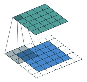
Convolutions with Padding!
- Padding is a technique used in CNNs to add extra border pixels to the input data before applying convolutions.
- Padding helps preserve spatial dimensions and avoid information loss at the edges of the input.
2. Benefits of Using Convolutions in deep learning
Convolutional Neural Networks (CNNs) is being used for many computer vision task. It is default neural network architecture when it comes to image classifications, object detection, image style transfer etc.
1. Supports Transfer Learning
Advantages:
- Fast adaptation: Significantly reducing training time and effort for related problems.
- Robust: We make the early layers more robust as they have essentially learned from multiple datasets rather than one, and more data means less overfitting to train dataset.
- Flexibility: Allows for rapid application in a variety of domains, such as medicine, autonomous vehicles, and robotics.
2. Parameter Sharing (Weight Reuse)
Example
If your image of size is
Compare this to a standard dense layer, having 100 neurons, total number of parameters here is
Advantages:
- Efficient computation: Reduces memory and computation overhead compared to fully connected layers.
- Generalization: Learned filters are applied throughout the input, improving overall generalization and robustness.
3. Translation Invariance
Example
A cat is still a cat regardless of whether it appears in the top half or the bottom half of the image. If a cat feature exists anywhere in the frame, the filter will activate.
Visual Example
In the below figure, the CNN filter is trained to detect the letter ‘C’ in the input image.
So lets input an image of letter ‘C’.
Now lets shift the letter ‘C’ down in the image by 1 pixel length.
4. Automatic, Hierarchical Feature Extraction
Advantages:
- Saves time and effort: Removes the dependency on domain-specific expertise for feature selection.
- Scalable representation learning: Can represent complex patterns with multiple layers of abstraction.
- Model flexibility: Works well for diverse tasks, including complex ones like scene understanding or video summarization.
5. Preservation of Spatial Relationships (Local Connectivity)
Advantages:
- Edge and texture recognition: Exploits spatial relationships between pixels in images.
- High accuracy: Performs exceptionally well in image classification, object detection, and segmentation tasks.
6. Reduced Overfitting
The shared weights and hierarchical feature extraction reduce model complexity compared to fully connected layers, thereby lowering the risk of overfitting.
Advantages:
- Better scalability: Handles large-scale datasets with limited data efficiently.
- Improved data usage: Reduces the need for extremely large labeled datasets due to parameter efficiency.
7. Efficient with Large Inputs
CNNs are optimized to handle large high-dimensional inputs (e.g., 1024x1024 pixel images) without overwhelming computational resources.
Advantages:
- Reduces dimensionality: Extracts relevant features while reducing input complexity (via pooling layers).
- Scalable architecture: Capable of handling large datasets of images, videos, etc., without degradation in performance.
8. Wide Range of Architectures
Variants of CNN architectures exist for specific applications, such as object detection, semantic segmentation, or generative modeling.
Advantages:
- Customizable designs:
- ResNet: Residual connections to avoid gradient vanishing.
- U-Net: Semantic segmentation for medical imaging.
- YOLO/SSD: Real-time object detection.
- GANs: Generates high-quality synthetic images or improves image resolution.
9. Improved Robustness with Regularization
CNNs often integrate regularization techniques like dropout, batch normalization, and L2 regularization to stabilize training.
Advantages:
- Prevents overfitting: Regularization techniques help achieve better generalization.
- Efficient training: Converges smoothly even for complex architectures.
10. Versatility Across Domains
CNNs are versatile models that have revolutionized various industries beyond computer vision.
Advantages:
- Applications beyond images:
- Medical Diagnosis: Disease detection from MRI scans and X-rays.
- Autonomous Systems: Object recognition for self-driving cars.
- Natural Language Processing (CNN-based models): Sentiment analysis and text classifications.
- Finance: Fraud detection based on transaction activity.
- Retail: Product categorization and recommendations.
11. Ease of Deployment
CNN models can be deployed conveniently using frameworks like TensorFlow, PyTorch, Keras, and ONNX for inference on edge devices (e.g., smartphones or IoT systems).
Advantages:
- Scalable solutions: Enables real-world applications like facial recognition, motion tracking, and augmented reality.
- Edge device compatibility: Neural networks can be optimized for real-time systems (e.g., using TensorFlow Lite).
12. Handles Rotation and Translation
CNNs are robust to certain transformations (e.g., rotation, translation). This property stems from pooling and feature normalization layers.
Advantages:
- Improves invariance: Offers reliable predictions regardless of the orientation or position of objects in the input.
- Better for real-world tasks: Useful for applications like autonomous driving, where object orientation varies.
13. Supports Multi-Channel Data
CNNs can process multi-channel inputs efficiently (e.g., RGB images, video with temporal frames, etc.).
Advantages:
- Multi-modal data compatibility: Enables applications like combining video frames with audio for speech recognition or gesture tracking.
3. Stride
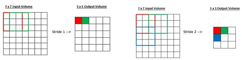
- Stride is a hyperparameter in Convolutional Neural Networks (CNNs) which determines the step size at which the convolutional filters (kernels) move across the input data. If we had stride 1 so it will take one by one. If we give stride 2 then it will take value by skipping the next 2 pixels.
- It controls the spatial displacement of the filters, impacting the output size and computational complexity.
Variations of Stride
- Stride of 1 (Standard Convolution): Extracting highly detailed, dense features without losing spatial resolution.
- Stride Greater Than 1 (Strided Convolution): In this the filter jumps by 2, 3, or more pixels at a time. Reducing the spatial dimensions of the feature map (downsampling).
- Asymmetric Stride: Using different stride values for the horizontal and vertical axes.
Advantages of Larger Strides (Stride > 1)
- Reduces Computational Load: Convolutions produce much smaller output feature maps. This drastically reduces the number of operations and memory required in subsequent layers.
- Increases Receptive Field: Moving the filter in larger jumps allows the network to "see" a wider area of the original image much faster. Subsequent layers will have a broader contextual understanding of the image.
- Fully Differentiable Downsampling: Unlike max pooling (which simply forces the network to drop non-maximum values), using a convolutional layer with a stride of 2 allows the network to learn its own weights for downsampling. This often leads to better model accuracy.
Disadvantages of Larger Strides
- Loss of Fine-Grained Information: You inevitably lose granular spatial details. If a crucial micro-feature falls into the "skipped" space, the network might miss it.
- Checkerboard Artifacts (in Generative Models): When generating images (upsampling), poorly tuned strides in "transposed convolutions" can cause uneven overlapping. This results in highly visible, repeating checkerboard patterns in the final generated image.
- Tuning Complexity: Finding the right balance between stride, filter size, and padding requires careful architectural design to ensure the output dimensions shrink at the correct mathematical rate.
In many modern architectures (like ResNet), a convolution layer with a stride of 2 is used instead of a max-pooling layer to reduce the image size while letting the network learn the best way to summarize the data.
Usecase
- Used to reduce dimension or compress the image.
- Stride greater than 1 also decreases the computation (Passive advantage)
Example: 2D Convolution with Stride
4. Pooling
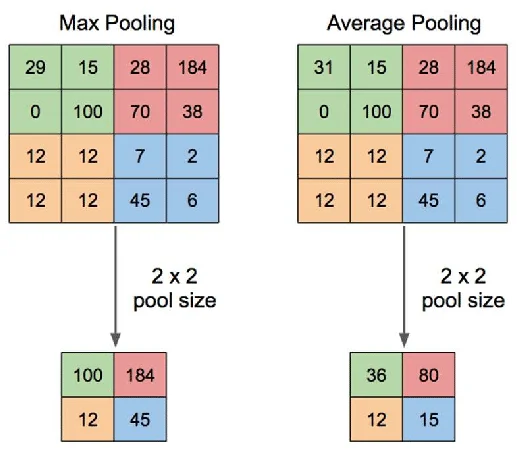
- Pooling is a downsampling operation commonly used in Convolutional Neural Networks (CNNs) to reduce the spatial dimensions of feature maps while retaining important information. This is also known as subsampling or downsampling.
- After a convolutional layer extracts features from an image, a pooling layer is often applied to summarize the presence of those features in patches. It does this by sliding a small window (usually 2x2 or 3x3) across the feature map and applying a mathematical operation to aggregate the values within that window.
Types of Pooling
-
Max Pooling: Extracting the most prominent or dominant features, such as sharp edges, lines, and corners. It is the most widely used pooling method in modern CNNs.
-
Average Pooling: It calculates the average of all the values in the region covered by the filter. Retaining background information and smoothing out the image. It is often used when the exact feature strength is less important than the overall presence of the feature.
-
Global Pooling (Global Average or Global Max): Instead of sliding a small window, global pooling takes the entire feature map (e.g., a 7x7 matrix) and reduces it to a single value (either the maximum or the average of the whole matrix). Best for: Drastically reducing dimensions right before the final classification layer, often replacing the need for traditional fully connected "flattening" layers.
Advantages
- Reduces Computational Cost: Pooling significantly reduces the number of parameters and helps to make the learned features more robust to small spatial variations and reduces computational complexity.
- Controls Overfitting: Because pooling removes detailed, pixel-perfect information and extracts only the broader summary of features, it helps prevent the model from memorizing the training data.
- Translation Invariance: Pooling makes the network robust to small shifts or translations in the input image. For example, if a cat's ear shifts a few pixels to the left, max pooling will still detect the "edge" of the ear within its window, allowing the network to recognize the object regardless of its exact position.
Disadvantages of Pooling
What are advantages can also be disadvantages like
-
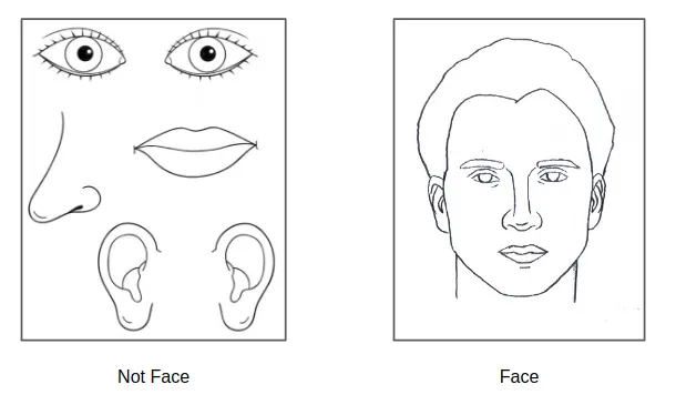
Loss of Spatial Information: By downsampling, the network loses spatial relation between different features. While it knows a feature exists, it loses the exact coordinates, which can be detrimental for tasks requiring pixel-perfect accuracy (like image segmentation).
This happens because the max pooling layer is applied to the outputs of each filter from previous convolution layer separately. Due to separately applying max pooling on each filter, much of the relative positional information between features is lost. So next layer can only give output based on the presence of features. As we go to subsequent layers, more and more of the spatial information is lost, as max pooling layer compunds the effect of translation invariance. In the end it detects a face even when the eye is present in the place of the mouth.
-
Destroys Fine Details: Max pooling, in particular, throws away up to 75% of the data (in a standard 2x2 stride 2 setup) simply by ignoring non-maximum values. In complex images, vital subtle details might be discarded entirely.
Where is Pooling Applied?
- Pool is applied on the output of convolution
5. Flatten
In a CNN, flattening is the process of converting a multi-dimensional feature map into a single, one-dimensional (1D) array or vector. The flattened acts as a bridge between the ➀ feature extraction part of the network (the convolutional and pooling layers) and ➁ the classification part of the network (the fully connected or dense layers).
Pros
- Retains all extracted feature data for the Dense layer to analyze.
Cons - Leads to millions of parameters in the Dense layers, making the model prone to overfitting and heavy to run.
6. Dropout
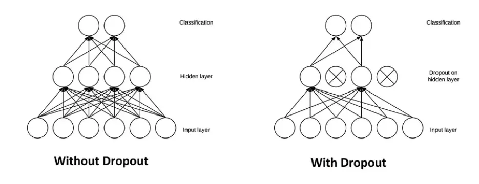
Dropout is a powerful regularization technique used in neural networks, including Convolutional Neural Networks (CNNs), to prevent the model from memorizing the training data (overfitting).
Because the network cannot rely on any single neuron being active, it forces the model to distribute its learning across the entire network. I. The Dropout layer is a mask that nullifies the contribution of some neurons toward the next layer and leaves all others.
Press enter or click to view image in full size
Why is Dropout Important?
- Prevents Overfitting: Deep CNNs have millions of parameters (as seen in the AlexNet example), making them prone to memorizing the training data. Dropout forces the network to generalize rather than memorize.
- Reduces Co-adaptation: Sometimes, neurons begin to rely too heavily on the outputs of specific neighboring neurons, essentially acting as a crutch. Dropout breaks these dependencies, forcing each neuron to learn useful, independent features.
- Simulates an Ensemble: Training with dropout is mathematically similar to training thousands of slightly different, smaller neural networks and averaging their predictions. Ensembles generally perform better and are more robust than single models.
Types of Dropout
1. Standard Dropout:
- Randomly zeros out individual neurons independently.
- Usually applied only to the Fully Connected (FC) layers at the very end of a CNN. Applying standard dropout to convolutional layers is often ineffective because adjacent pixels in a feature map are highly correlated; if one pixel is dropped, the network can just infer the missing information from its neighbors.
2. Spatial Dropout (Channel Dropout)
- Instead of dropping individual pixels (neurons) within a feature map, Spatial Dropout randomly drops the entire 2D feature map (an entire channel).
- Excellent for convolutional layers. It forces the network to look for different features entirely rather than relying on a specific channel (like an edge detector) being present.
3. DropBlock
- Drops a contiguous square block of neurons across the feature map, rather than dropping independent pixels or entire channels.
- Highly effective for modern convolutional layers. It removes a large enough spatial region that the network cannot simply guess the missing information from immediate neighboring pixels, forcing it to look at other regions of the image.
4. Alpha Dropout
- A specialized form of dropout designed specifically to be used with the SELU (Scaled Exponential Linear Unit) activation function.
- Used in Self-Normalizing Neural Networks (SNNs). It ensures that the mean and variance of the inputs are preserved after the dropout is applied, keeping the network mathematically stable.
7. Activation Function
Refer 👉 Activation Function
8. Filters
Refer 👉 Computer Vision - Filters
As we move along the network of CNN, we loose spatial information But we are able to gain global (high level) information of image, which make its very useful in classification. In classification you don't need to know where in the image, object of interest lies, but only need to know what that object is.
🤔💭 Questions and Answers
1. Parameters vs. Hyperparameters in CNNs
In any neural network, including CNNs, there is a strict dividing line between what the model learns on its own (parameters) and what can be programmed (hyperparameters).
| Feature | Parameters | Hyperparameters |
|---|---|---|
| Definition | Internal variables that the model learns and adjusts automatically during training. | External configurations set manually by the architect before training begins. |
| How they change | Continuously updated via backpropagation and gradient descent to minimize error. | Static during a training run. They are only changed manually between runs to find a better configuration. |
| CNN Examples | The weights inside a convolutional filter, the biases added to a feature map, the weights in fully connected layers. | Learning rate, batch size, number of epochs, filter size (e.g., 3x3), stride size, pooling type (max/average). |
2. Pooling vs. Strides
Both pooling layers and strided convolutions (using a stride
While the end result—a smaller feature map—is similar, the mechanics and implications are different:
-
Pooling is an explicit, fixed mathematical operation (like taking the maximum or average value) applied to a region after a convolution has already happened. It contains zero learnable parameters. It forces the network to summarize.
-
Strided Convolution combines feature extraction and downsampling into a single step. By skipping pixels (e.g., using a stride of 2), the convolutional filter naturally outputs a smaller feature map. Because this is a convolutional layer, the network uses its parameters (weights) to actually learn the best way to downsample the image.
3. When to Choose Which?
Choose Pooling when:
- Max pooling is excellent at ensuring that slight shifts in the input image do not drastically alter the output, which is great for standard classification tasks.
- Max pooling aggressively throws away non-maximum data, forcing the network to focus only on the most dominant features (like strong edges or textures).
- Pooling requires zero parameters and uses very simple math, making it computationally cheaper than adding another convolutional layer.
Choose Strided Convolutions when:
- You want the network to learn the downsampling: Instead of throwing away data using a hardcoded rule (like max pooling), strided convolutions let the network optimize its own weights to figure out exactly what information is important to keep while shrinking the image.
- You are building modern architectures: Networks like ResNet rely heavily on strided convolutions rather than max pooling to preserve more complex spatial relationships throughout the network.
- You are building Generative Models: In models that generate images (like GANs or Variational Autoencoders), pooling operations can cause significant information loss that makes it hard for the network to reconstruct high-quality images later. Strided convolutions are almost always preferred here.
4. Flattening vs. Global Pooling
In older, classic CNN architectures (like VGG16 or AlexNet), flattening was the standard way to transition to the final classification layers. However, modern architectures often replace the Flatten layer with Global Average Pooling (GAP).
| Feature | Flatten | Global Average Pooling (GAP) |
|---|---|---|
| Mechanics | Convert all the resultant 2D or 3D arrays from pooled feature maps into a single long continuous linear vector. | Averages the entire spatial dimensions of each channel into a single number. |
| Output Size | Usually massive (e.g., 7x7x512 becomes an array of 25,088 values). | Much smaller (e.g., 7x7x512 becomes an array of just 512 values). |
| Pros | Retains all extracted feature data for the Dense layer to analyze. | Drastically reduces parameters, saving computational power and preventing overfitting. |
| Cons | Leads to millions of parameters in the Dense layers, making the model prone to overfitting and heavy to run. | Destroys all spatial layout information, though usually acceptable at the very end of the network. |
5. What is the typical workflow of CNN and when and how are weights in kernel updated?
Here is how the flow works in reality.
Step 1: The Forward Pass (Predicting)
During training, the network takes an image and pushes it through all the layers. At the very end, it makes a prediction (e.g., "I am 80% sure this is a dog").
The network then calculates the Loss (how wrong that prediction was compared to the actual label).
At this exact moment, the weights have not been updated yet. The network just holds onto the math of "how wrong" it was.
Step 2: The Backward Pass (Calculating the Fixes)
The network works backward from the end to the beginning (Backpropagation), calculating exactly how much each kernel and filter needs to change to make a better prediction next time. It calculates these "fixes" (gradients), but again, it does not apply them yet.
Step 3: The Weight Update (When it actually happens)
When those fixes are actually applied to the kernels is dictated by the Batch Size you set for your Optimizer.
Here are the three scenarios for when the updates happen:
Scenario A: Batch Size = 1 (Stochastic Gradient Descent)
- The Flow: Image 1 goes through -> Loss calculated -> Fixes calculated -> Weights updated. * Then, Image 2 goes through the newly updated network -> Loss calculated -> Fixes calculated -> Weights updated.
- Result: The weights are updated after each individual image.
Scenario B: Batch Size = Total
- The Flow: All
images are pushed through the network one by one. The network calculates the fixes for Image 1, then Image 2, all the way to Image , and keeps a running tally of them in its memory. - Once all
images are processed, it averages all those fixes together and makes one single massive weight update. - Result: The weights are updated only after all images are processed.
Scenario C: Batch Size = 32 (Mini-Batch SGD — The Standard)
- The Flow: The network processes a "chunk" of 32 images. It calculates the loss and the required fixes for all 32 images, averages those fixes together, and then updates the weights.
- Then it grabs the next chunk of 32 images, repeats the process, and updates the weights again.
- Result: The weights are updated after every chunk of images.