Complete Forward & Backward Propagation Example

Overview: The Big Picture

Phase	Purpose	Key Output
Forward Propagation	Pass input through the network to get a prediction	Prediction $\hat{y}$ and Loss $L$
Backward Propagation	Compute gradients — how much each weight contributed to the error	Gradients $\frac{\partial L}{\partial w}$ for all weights
Weight Update	Adjust weights to reduce the error	New weights $w_{n e w}$

One complete cycle (Forward → Backward → Update) = One Training Iteration
Repeat for many iterations (epochs) until the loss is minimized and predictions are accurate.

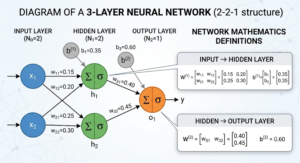
Network Architecture

Input Layer (2 neurons) → Hidden Layer (2 neurons) → Output Layer (1 neuron)

Activation Function (Hidden): Sigmoid: $σ (z) = \frac{1}{1 + e^{- z}}$
Activation Function (Output): Sigmoid
Loss Function: Binary Cross-Entropy (BCE): $L = - [y \log (\hat{y}) + (1 - y) \log (1 - \hat{y})]$

Notation Reference

Symbol	Meaning
$x_{i}$	Input feature $i$
$w_{i j}$	Weight from input $i$ to hidden neuron $j$
$w_{3 j}$	Weight from hidden neuron $j$ to output
$b_{j}$	Bias for neuron $j$
$z_{j}^{(l)}$	Pre-activation (weighted sum) at layer $l$ , neuron $j$
$a_{j}^{(l)}$	Activation (output after sigmoid) at layer $l$ , neuron $j$
$\hat{y}$	Network's prediction (output layer activation)
$y$	True target label
$L$	Loss (error)
$δ_{j}^{(l)}$	Error signal at layer $l$ , neuron $j$
$η$	Learning rate

Sample Data (5 rows, 2 columns)

Sample	$x_{1}$	$x_{2}$	$y$ (Target)
1	0.1	0.2	0
2	0.4	0.5	1
3	0.3	0.6	1
4	0.7	0.1	0
5	0.9	0.8	1

Initialized Weights and Biases

Input → Hidden Layer:

W^{(1)} = [\begin{matrix} w_{11} & w_{12} \\ w_{21} & w_{22} \end{matrix}] = [\begin{matrix} 0.15 & 0.20 \\ 0.25 & 0.30 \end{matrix}] b^{(1)} = [\begin{matrix} b_{1} \\ b_{2} \end{matrix}] = [\begin{matrix} 0.35 \\ 0.35 \end{matrix}]

Hidden → Output Layer:

W^{(2)} = [\begin{matrix} w_{31} & w_{32} \end{matrix}] = [\begin{matrix} 0.40 & 0.45 \end{matrix}] b^{(2)} = 0.60

Diagrammatic Representation

👉 Both Forward and Backward Propagation is detailed for Sample 1: $x_{1} = 0.1$ , $x_{2} = 0.2$ , $y = 0$

Forward Propagation

5-Step Forward Propagation Steps

Step 1: Input to Hidden Layer

Compute weighted sum ( $z$ ) for each hidden neuron:

\begin{aligned} (Linear Equation) & z_{1}^{(1)} = w_{11} \cdot x_{1} + w_{21} \cdot x_{2} + b_{1} \\ z_{1}^{(1)} & = 0.15 \times 0.1 + 0.25 \times 0.2 + 0.35 = 0.015 + 0.05 + 0.35 = 0.415 \\ z_{2}^{(1)} = w_{12} \cdot x_{1} + w_{22} \cdot x_{2} + b_{2} \\ z_{2}^{(1)} & = 0.20 \times 0.1 + 0.30 \times 0.2 + 0.35 = 0.02 + 0.06 + 0.35 = 0.43 \end{aligned}

Step 2: Apply sigmoid activation:

》Sigmoid

\begin{aligned} a_{1}^{(1)} & = σ (z_{1}^{(1)}) = σ (0.415) = \frac{1}{1 + e^{- 0.415}} = 0.6023 \\ a_{2}^{(1)} & = σ (z_{2}^{(1)}) = σ (0.43) = \frac{1}{1 + e^{- 0.43}} = 0.6058 \end{aligned}

Step 3: Hidden to Output Layer

Compute weighted sum for output:

\begin{aligned} z^{(2)} & = w_{31} \cdot a_{1}^{(1)} + w_{32} \cdot a_{2}^{(1)} + b^{(2)} \\ z^{(2)} & = 0.40 \times 0.6023 + 0.45 \times 0.6058 + 0.60 \\ z^{(2)} & = 0.2409 + 0.2726 + 0.60 = 1.1135 \end{aligned}

Step 4: Apply sigmoid activation (final prediction)

\hat{y} = a^{(2)} = σ (z^{(2)}) = σ (1.1135) = \frac{1}{1 + e^{- 1.1135}} = \frac{1}{1.3285} = 0.7528

Step 5: Calculate Loss (Binary Cross-Entropy)

》Binary Cross-Entropy

\begin{aligned} L = - [y \log (\hat{y}) + (1 - y) \log (1 - \hat{y})] \\ (For Sample 1 where y = 0) & L & = - [0 \cdot \log (0.7528) + (1 - 0) \cdot \log (1 - 0.7528)] \\ L & = 1.3976 \end{aligned}

$\dots$ Iterate the process for all the rows

Forward Propagation Results for All 5 Samples

Sample	$x_{1}$	$x_{2}$	$z_{1}^{(1)}$	$z_{2}^{(1)}$	$a_{1}^{(1)}$	$a_{2}^{(1)}$	$z^{(2)}$	$\hat{y}$	$y$	BCE Loss
1	0.1	0.2	0.415	0.430	0.6023	0.6058	1.1135	0.7528	0	1.3976
2	0.4	0.5	0.535	0.580	0.6307	0.6411	1.1407	0.7757	1	0.2538
3	0.3	0.6	0.545	0.590	0.6330	0.6434	1.1428	0.7760	1	0.2534
4	0.7	0.1	0.480	0.520	0.6177	0.6272	1.1293	0.7737	0	1.4858
5	0.9	0.8	0.685	0.770	0.6649	0.6836	1.1734	0.8282	1	0.1884

Total BCE Loss:

\begin{aligned} L_{t o t a l} = \frac{1}{N} \sum_{i = 1}^{N} L_{i} \\ L_{t o t a l} & = \frac{1}{5} (1.3976 + 0.2538 + 0.2534 + 1.4858 + 0.1884) = \frac{3.5790}{5} \\ L_{t o t a l} & = 0.7261 \end{aligned}

Backward Propagation

We compute gradients using the chain rule and propagate errors backward.

\begin{array}{r} \frac{\partial L}{\partial w} = \frac{\partial L}{\partial \hat{y}} \cdot \frac{\partial \hat{y}}{\partial z^{(2)}} \cdot \frac{\partial z^{(2)}}{\partial a^{(1)}} \cdot \frac{\partial a^{(1)}}{\partial z^{(1)}} \cdot \frac{\partial z^{(1)}}{\partial w^{(1)}} \end{array}

Visual Representation of Backpropagation

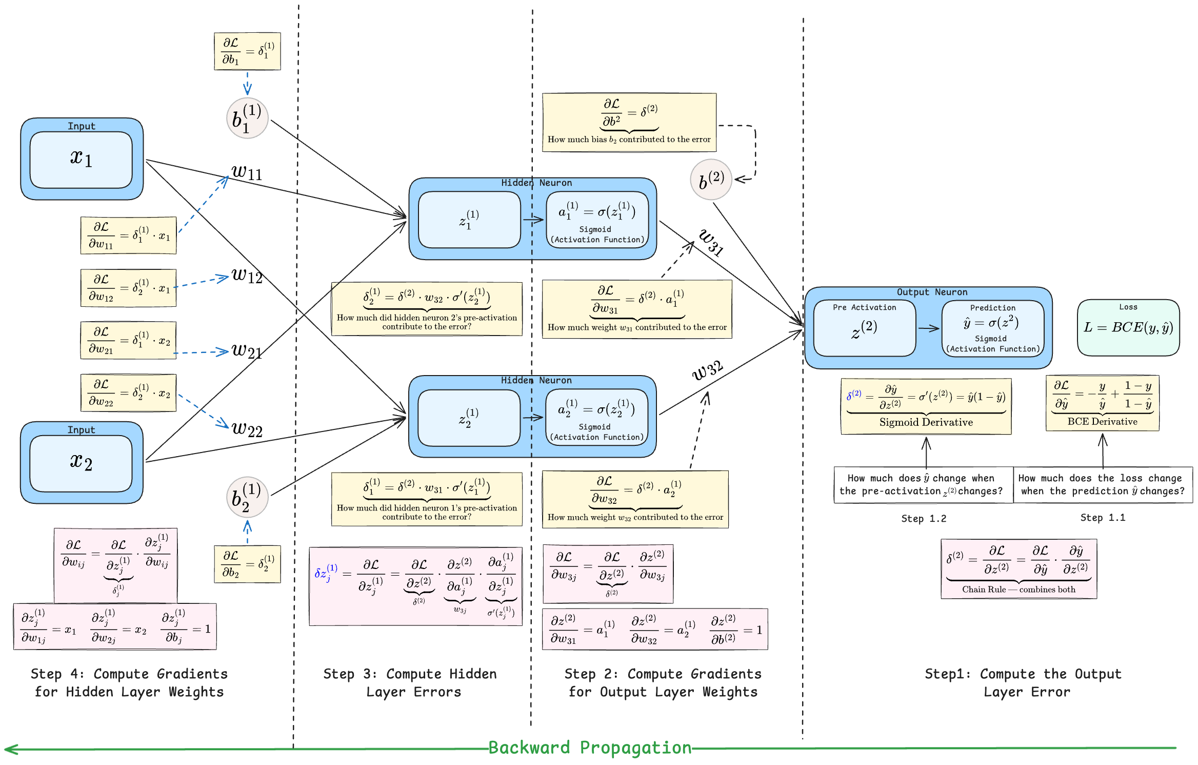
5-Step Backward Propagation Steps

Step 1: Compute the Output Layer Error

Goal

This error signal tells us the "blame" assigned to the output neuron ( $δ^{(2)}$ ), which we'll use to update its weights and propagate backward.
How — Calculate the error at the output neuron by finding $^{(1)}$ the difference between the actual target and the prediction, $^{(2)}$ scaled by the derivative of its activation function.

Step 1.1 — Binary Cross-Entropy Derivative:

👉 Question — How much does the loss change when the prediction $\hat{y}$ changes?
➢ This measures the sensitivity of our loss function to prediction errors. If the prediction is far from the truth, this value is large.

\frac{\partial L}{\partial \hat{y}} = σ^{'} (\hat{y}) = - \frac{y}{\hat{y}} + \frac{1 - y}{1 - \hat{y}} = - \frac{0}{0.7528} + \frac{1}{0.2472} = 4.0453

Step 1.2 — Sigmoid Derivative:

Question — How much does $\hat{y}$ change when the pre-activation $z^{(2)}$ changes?
➢ This captures magnitude — how "steep" the sigmoid curve is at the current output. The slope is largest near $\hat{y} = 0.5$ and flattest near $\hat{y} = 0$ or $\hat{y} = 1$ .

\frac{\partial \hat{y}}{\partial z^{(2)}} = σ^{'} (z^{(2)}) = \hat{y} (1 - \hat{y}) = 0.7528 \times 0.2472 = 0.1861

Step 1.3 — The Output Neuron Error ( $δ^{(2)}$ ):

Question — How the loss changes with the pre-activation $z^{(2)}$ .
➢ It acts as the primary scaling factor, dictating the overall direction and magnitude of the necessary correction at the end of the network.

Calculation: The Multiplication (Chain Rule)

\begin{aligned} δ^{(2)} & = \frac{\partial L}{\partial z^{(2)}} = \frac{\partial L}{\partial \hat{y}} \cdot \frac{\partial \hat{y}}{\partial z^{(2)}} \end{aligned}

We can see the calculations in 2 ways

Method 1: Substitution:

When you substitute (i) and (ii) and simplify, a remarkably clean result emerges:

\begin{aligned} δ^{(2)} & = \frac{\partial L}{\partial z^{(2)}} = \frac{\partial L}{\partial \hat{y}} \cdot \frac{\partial \hat{y}}{\partial z^{(2)}} \\ δ^{(2)} & = 4.0453 \times 0.1861 \\ δ^{(2)} & = 0.7528 \end{aligned}

Method 2: Equation Simplification

\begin{aligned} (chain rule) & δ^{(2)} = \frac{\partial L}{\partial z^{(2)}} = \frac{\partial L}{\partial \hat{y}} \cdot \frac{\partial \hat{y}}{\partial z^{(2)}} \\ δ^{(2)} & = (- \frac{y}{\hat{y}} + \frac{1 - y}{1 - \hat{y}}) \cdot \hat{y} (1 - \hat{y}) \\ δ^{(2)} & = - y + y \hat{y} + \hat{y} - y \hat{y} \\ δ^{(2)} = \hat{y} - y \\ (y=0) & δ^{(2)} & = 0.7528 - 0 \\ δ^{(2)} = 0.7528 \end{aligned}

This elegant result makes implementation much simpler!

This isn't a coincidence — BCE was designed specifically to pair with sigmoid. The "ugly" fractions in the BCE derivative perfectly cancel with the sigmoid derivative, giving us the clean $\hat{y} - y$ result.

Step 2: Gradients for Output Layer Weights

Goal

Find $\frac{\partial L}{\partial w_{31}}$ , $\frac{\partial L}{\partial w_{32}}$ , $\frac{\partial L}{\partial b^{(2)}}$ ➛ How much does each output-layer weights, the bias, or the activations from the previous layer contribute to the loss?
These gradients tell us how much a specific weight connecting the hidden layer to the output layer needs to adjust and by how much to reduce the error.

Recap

Recall that $z^{(2)} = w_{31} \cdot a_{1}^{(1)} + w_{32} \cdot a_{2}^{(1)} + b^{(2)}$ .

The hidden activation $a_{1}^{(1)}$ and $a_{2}^{(1)}$ is the input flowing into weight $w_{31}$ and $w_{32}$ respectively.
A larger input means that weight had more influence on the output — so it deserves more "blame" for the error.

The Chain Rule for Each Parameter
Each gradient is found by extending the chain rule one more step — from z⁽²⁾ back to the weight:

\begin{aligned} \frac{\partial L}{\partial w_{3 j}} = \underset{δ^{(2 >)}}{\underset{⏟}{\frac{\partial L}{\partial z^{(2)}}}} \cdot \frac{\partial z^{(2)}}{\partial w_{3 j}} \end{aligned}

Local derivatives are simply:

\begin{aligned} \frac{\partial z^{(2)}}{\partial w_{31}} = a_{1}^{(1)} & \frac{\partial z^{(2)}}{\partial w_{32}} = a_{2}^{(> 1)} & \frac{\partial z^{(2)}}{\partial b^{(2)}} = 1 \end{aligned}

The Three Gradients

Gradient for weight $w_{31}$

Question—How much weight $w_{31}$ contributed to the error?

\begin{array}{r} \frac{\partial L}{\partial w_{31}} = δ^{(2)} \cdot a_{1}^{(1)} = 0.7528 \times 0.6023 = 0.4533 \end{array}

Gradient for weight $w_{32}$

Question—How much weight $w_{32}$ contributed to the error?

\begin{array}{r} \frac{\partial L}{\partial w_{32}} = δ^{(2)} \cdot a_{2}^{(1)} = 0.7528 \times 0.6058 = 0.4561 \end{array}

Gradient for bias $b_{2}$

Question—How much Bias $b^{(2)}$ contributed to the error?
Bias has no input multiplier, just the error

\begin{array}{r} \frac{\partial L}{\partial b^{(2)}} = δ^{(2)} = 0.7528 \end{array}

Key insight — Gradient = Error × Input

A weight's gradient depends on two things:
- The output error ( $δ^{(2)}$ ) — how wrong the network was.
- The incoming activation ( $a_{j}^{(1)}$ ) — how active that connection was.
  - If a hidden neuron's activation (aⱼ⁽¹⁾) is large, its weight gets a bigger adjustment, because it was more "responsible" for the output.
  - If the activation is near zero, that weight barely changes — it had little influence.

Step 3: Hidden Layer Errors

Goal

Find $\frac{\partial L}{\partial z_{1}^{(1)}}$ and $\frac{\partial L}{\partial z_{2}^{(1)}}$ ➛ How much does each hidden neuron's pre-activation contribute to the loss?
These error signals tell us how much "blame" each hidden neuron deserves, which we'll use to update the input-to-hidden weights.

Recap

Recall that $z^{(2)} = w_{31} \cdot a_{1}^{(1)} + w_{32} \cdot a_{2}^{(1)} + b^{(2)}$ and $a_{j}^{(1)} = σ^{'} (z_{j}^{(1)})$ .

The weight $w_{3 j}$ determines how much hidden neuron $j$ influences the output.
A larger weight means that hidden neuron had more influence on the output — so it deserves more "blame" for the error.

The Chain Rule for Each Parameter
Each hidden error is found by extending the chain rule two more steps — from $z^{(2)}$ back through the activation $a_{j}^{(1)}$ to the pre-activation $z_{j}^{(1)}$ :

\begin{aligned} \frac{\partial L}{\partial z_{j}^{(1)}} = \underset{δ^{>} (2)}{\underset{⏟}{\frac{\partial L}{\partial z^{(2)}}}} \cdot \underset{w_{3 j}}{\underset{⏟}{\frac{\partial z^{(2)}}{\partial a_{j}^{(1)}}}} \cdot \underset{σ^{'} (z_{j}^{(1)})}{\underset{⏟}{\frac{\partial a_{j}^{(1)}}{\partial z_{j}^{(1)}}}} \end{aligned}

Since $z^{(2)} = w_{31} a_{1}^{(1)} + w_{32} a_{2}^{(1)} + b^{(2)}$ and $a_{j}^{(1)} = σ^{'} (z_{j}^{(1)})$ , the local derivatives are:

\begin{aligned} \frac{\partial z^{(2)}}{\partial a_{1}^{(1)}} = w_{31} & \frac{\partial z^{(2)}}{\partial a_{2}^{(1)}} = w_{32} & \frac{\partial a_{j}^{(1)}}{\partial z_{j}^{(1)}} = a_{j}^{(1)} (1 - a_{j}^{(1)}) \end{aligned}

This simplifies to the general formula:

δ_{j}^{(1)} = (δ^{(2)} \cdot w_{3 j}) \cdot σ^{'} (z_{j}^{(1)})

The Two Hidden Error Signals

Term	What it represents	Value
$δ^{(2)}$	Output error (already computed in Step 1)	$0.7528$ (From Step 2)
$w_{31}$	Connection strength from hidden neuron 1 to output	$0.40$ (Input Assumption)
$w_{32}$	Connection strength from hidden neuron 2 to output	$0.45$ (Input Assumption)
$σ^{'} (z_{1}^{(1)})$	Sigmoid derivative — how "responsive" neuron 1 was	$a_{1}^{(1)} (1 - a_{1}^{(1)}) = 0.2395$
$σ^{'} (z_{2}^{(1)})$	Sigmoid derivative — how "responsive" neuron 2 was	$a_{2}^{(1)} (1 - a_{2}^{(1)}) = 0.2387$

Error for hidden neuron 1 ( $δ_{1}^{(1)}$ )

Question — How much did hidden neuron 1's pre-activation contribute to the error?

\begin{aligned} δ_{1}^{(1)} & = δ^{(2)} \cdot w_{31} \cdot σ^{'} (z_{1}^{(1)}) \\ = 0.7528 \times 0.40 \times 0.2395 \\ δ_{1}^{(1)} = 0.0721 \end{aligned}

Error for hidden neuron 2 ( $δ_{2}^{(1)}$ )

Question — How much did hidden neuron 2's pre-activation contribute to the error?

\begin{aligned} δ_{2}^{(1)} & = δ^{(2)} \cdot w_{32} \cdot σ^{'} (z_{2}^{(1)}) \\ = 0.7528 \times 0.45 \times 0.2387 \\ δ_{2}^{(1)} = 0.0809 \end{aligned}

Key Insight — Hidden Error = Output Error × Weight × Local Slope

A hidden neuron's error depends on three things:
- The output error ( $δ^{(2)}$ ) — how wrong the network was overall.
- The connection weight ( $w_{3 j}$ ) — how strongly this neuron influenced the output.
- The activation slope ( $σ^{'}$ ) — how responsive this neuron was at its current input.
If a neuron was strongly connected and highly responsive, it receives more blame and will be adjusted more.
If the sigmoid is saturated (output near 0 or 1), $σ^{'} \approx 0$ , so very little error flows backward — this is the vanishing gradient problem.

Step 4: Gradients for Hidden Layer Weights

Goal

Find $\frac{\partial L}{\partial w_{11}}$ , $\frac{\partial L}{\partial w_{21}}$ , $\frac{\partial L}{\partial w_{12}}$ , $\frac{\partial L}{\partial w_{22}}$ , $\frac{\partial L}{\partial b_{1}}$ , $\frac{\partial L}{\partial b_{2}}$ ➛ How much does each input-to-hidden weight and bias contribute to the loss?
These gradients tell us how to adjust the connections between the input layer and the hidden layer to reduce the error.

Recap

Recall that $z_{j}^{(1)} = w_{1 j} \cdot x_{1} + w_{2 j} \cdot x_{2} + b_{j}$ .

The input $x_{i}$ is the value flowing into weight $w_{i j}$ .
A larger input means that weight had more influence on the hidden neuron's output — so it deserves more "blame" for the error.

The Chain Rule for Each Parameter
Since we already computed $δ_{j}^{(1)} = \frac{\partial L}{\partial z_{j}^{(1)}}$ in Step 3, we just need one more link in the chain:

\begin{aligned} \frac{\partial L}{\partial w_{i j}} = \underset{δ_{j}^{(1)}}{\underset{⏟}{\frac{\partial L}{\partial z_{j}^{(1)}}}} \cdot \frac{\partial z_{j}^{(1)}}{\partial w_{i j}} \end{aligned}

Since $z_{j}^{(1)} = w_{1 j} \cdot x_{1} + w_{2 j} \cdot x_{2} + b_{j}$ , the local derivatives are simply:

\begin{aligned} \frac{\partial z_{j}^{(1)}}{\partial w_{1 j}} = x_{1} & \frac{\partial z_{j}^{(1)}}{\partial w_{2 j}} = x_{2} & \frac{\partial z_{j}^{(1)}}{\partial b_{j}} = 1 \end{aligned}

The Six Gradients

Term	What it represents	Value
$δ_{1}^{(1)}$	Hidden neuron 1 error (from Step 3)	$0.0721$ (From Step 3)
$δ_{2}^{(1)}$	Hidden neuron 2 error (from Step 3)	$0.0809$ (From Step 3)
$x_{1}$	Input feature 1	$0.1$ (Input Assumption)
$x_{2}$	Input feature 2	$0.2$ (Input Assumption)

Gradient for weight $w_{11}$

Question — How much did weight $w_{11}$ (connecting $x_{1}$ to hidden neuron 1) contribute to the error?

\begin{aligned} \frac{\partial L}{\partial w_{11}} & = δ_{1}^{(1)} \cdot x_{1} \\ = 0.0721 \times 0.1 \\ \frac{\partial L}{\partial w_{11}} = 0.00721 \end{aligned}

Gradient for weight $w_{21}$

Question — How much did weight $w_{21}$ (connecting $x_{2}$ to hidden neuron 1) contribute to the error?

\begin{aligned} \frac{\partial L}{\partial w_{21}} & = δ_{1}^{(1)} \cdot x_{2} \\ = 0.0721 \times 0.2 \\ \frac{\partial L}{\partial w_{21}} = 0.01442 \end{aligned}

Gradient for weight $w_{12}$

Question — How much did weight $w_{12}$ (connecting $x_{1}$ to hidden neuron 2) contribute to the error?

\begin{aligned} \frac{\partial L}{\partial w_{12}} & = δ_{2}^{(1)} \cdot x_{1} \\ = 0.0809 \times 0.1 \\ \frac{\partial L}{\partial w_{12}} = 0.00809 \end{aligned}

Gradient for weight $w_{22}$

Question — How much did weight $w_{22}$ (connecting $x_{2}$ to hidden neuron 2) contribute to the error?

\begin{aligned} \frac{\partial L}{\partial w_{22}} & = δ_{2}^{(1)} \cdot x_{2} \\ = 0.0809 \times 0.2 \\ \frac{\partial L}{\partial w_{22}} = 0.01618 \end{aligned}

Gradient for bias $b_{1}$

Question — How much did bias $b_{1}$ contribute to the error?
Bias has no input multiplier, just the error

\begin{aligned} \frac{\partial L}{\partial b_{1}} & = δ_{1}^{(1)} \\ \frac{\partial L}{\partial b_{1}} = 0.0721 \end{aligned}

Gradient for bias $b_{2}$

Question — How much did bias $b_{2}$ contribute to the error?
Bias has no input multiplier, just the error

\begin{aligned} \frac{\partial L}{\partial b_{2}} & = δ_{2}^{(1)} \\ \frac{\partial L}{\partial b_{2}} = 0.0809 \end{aligned}

Key Insight — Gradient = Error × Input (Same Pattern as Step 2!)

A weight's gradient depends on two things:
- The hidden neuron's error ( $δ_{j}^{(1)}$ ) — how much blame this neuron received.
- The incoming input ( $x_{i}$ ) — how active that input was.
If an input is large, the weights connected to it get bigger adjustments, because they had more influence.
This pattern — Gradient = Error × Input — repeats at every layer in deep networks, making backpropagation elegant and scalable.

Step 5: Weight Updates

Goal

Calculate new values of $w_{11}$ , $w_{21}$ , $w_{12}$ , $w_{22}$ , $w_{31}$ , $w_{32}$ , $b_{1}^{(1)}$ , $b_{2}^{(1)}$ , $b^{(2)}$
Using gradient descent:

$w_{n e w} = w_{o l d} - η \cdot \nabla w$
$b_{n e w} = b_{o l d} - η \cdot \frac{\partial L}{\partial b}$

Assumption
➢ Learning Rate $η = 0.5$

Weight	Old Value	Gradient	New Value
$w_{11}$	0.15	0.00721	0.1464
$w_{21}$	0.25	0.01442	0.2428
$w_{12}$	0.20	0.00809	0.1960
$w_{22}$	0.30	0.01618	0.2919
$b_{1}$	0.35	0.0721	0.3139
$b_{2}$	0.35	0.0809	0.3096
$w_{31}$	0.40	0.4533	0.1733
$w_{32}$	0.45	0.4561	0.2219
$b^{(2)}$	0.60	0.7528	0.2236

What Happens Next?

Repeat for all samples — In practice, you'd compute gradients for all 5 samples and average them (batch gradient descent), or update after each sample (stochastic gradient descent).
Multiple Epochs — One pass through all samples = 1 epoch. Training typically requires hundreds or thousands of epochs until loss converges.
Monitor Loss — After each epoch, check if $L_{t o t a l}$ is decreasing. If it plateaus or increases, adjust learning rate or check for issues.
Evaluate — Once trained, test on unseen data to measure generalization.

Key Insight: The beauty of backpropagation is that the same pattern — Gradient = Error × Input — repeats at every layer, making it computationally efficient and scalable to deep networks.

Complete Forward & Backward Propagation Example

Overview: The Big Picture

Network Architecture

Notation Reference

Sample Data (5 rows, 2 columns)

Initialized Weights and Biases

Diagrammatic Representation

Forward Propagation

5-Step Forward Propagation Steps

Step 1: Input to Hidden Layer

Step 2: Apply sigmoid activation:

Step 3: Hidden to Output Layer

Step 4: Apply sigmoid activation (final prediction)

Step 5: Calculate Loss (Binary Cross-Entropy)

Forward Propagation Results for All 5 Samples

Total BCE Loss:

Backward Propagation

Visual Representation of Backpropagation

5-Step Backward Propagation Steps

Step 1: Compute the Output Layer Error

Step 1.1 — Binary Cross-Entropy Derivative:

Step 1.2 — Sigmoid Derivative:

Step 1.3 — The Output Neuron Error (δ(2)):

Method 1: Substitution:

Method 2: Equation Simplification

Step 2: Gradients for Output Layer Weights

The Three Gradients

Gradient for weight w31

Gradient for weight w32

Gradient for bias b2

Key insight — Gradient = Error × Input

Step 3: Hidden Layer Errors

The Two Hidden Error Signals

Error for hidden neuron 1 (δ1(1))

Error for hidden neuron 2 (δ2(1))

Key Insight — Hidden Error = Output Error × Weight × Local Slope

Step 4: Gradients for Hidden Layer Weights

The Six Gradients

Gradient for weight w11

Gradient for weight w21

Gradient for weight w12

Gradient for weight w22

Gradient for bias b1

Gradient for bias b2

Key Insight — Gradient = Error × Input (Same Pattern as Step 2!)

Step 5: Weight Updates

What Happens Next?

Step 1.3 — The Output Neuron Error ( $δ^{(2)}$ ):

Gradient for weight $w_{31}$

Gradient for weight $w_{32}$

Gradient for bias $b_{2}$

Error for hidden neuron 1 ( $δ_{1}^{(1)}$ )

Error for hidden neuron 2 ( $δ_{2}^{(1)}$ )

Gradient for weight $w_{11}$

Gradient for weight $w_{21}$

Gradient for weight $w_{12}$

Gradient for weight $w_{22}$

Gradient for bias $b_{1}$

Gradient for bias $b_{2}$