Singular Value Decomposition (SVD)

The one-line intuition

Eigendecomposition rotates, stretches, and rotates back ( $A = Q Λ Q^{- 1}$ — same basis both sides).
SVD rotates from one basis, stretches, and rotates into a possibly different basis ( $A = U Σ V^{⊤}$ ). That freedom to use two different bases is exactly what lets SVD handle rectangular matrices.

Understanding Singular Value Decomposition (SVD)

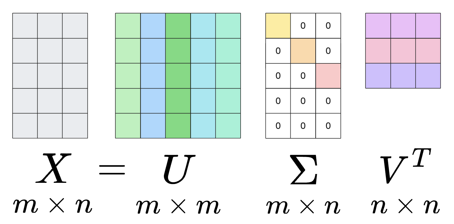
SVD is a powerful matrix decomposition technique that decomposes a matrix $A$ into three components to extract its fundamental structure and insights. For a given matrix $X$ (of size $m \times n$ ):

$U$ : Left Singular Vectors ( $m \times m$ )
- Columns of $U$ are orthogonal eigenvectors of the symmetric matrix $A A^{⊤}$ .
- Provides the directions of maximum variance among the row space (features) of $A$ .
$Σ$ : Singular Values ( $m \times n$ )
- A diagonal matrix containing the singular values ( $σ_{i}$ ) of $A$ . Singular values measure the "strength" or importance of each mode (principal component).
$V$ : Right Singular Vectors ( $n \times n$ )
- Columns of $V$ are orthogonal eigenvectors of the symmetric matrix $A^{⊤} A$ .
- Represents the Principal Components in the column space, or the directions where the data is most spread out.

Each of these components has a specific role in describing the structure and action of the matrix.

1. Left Singular Vectors ( $U$ from $A A^{T}$ )

Mathematical Insight:

The columns of $U$ are called left singular vectors ( $u_{i}$ );
They are orthogonal eigenvectors of the symmetric matrix $A A^{⊤}$ .

Role:

$U$ captures the relationships (covariance relationships) among the rows of $A$ (row-space).
If the rows represent features of data points, $U$ identifies the directions of maximum variance among the row-space of the data.

Properties:

Orthogonality: All left singular vectors are orthogonal ( $u_{i} ⊥ u_{j}$ for $i \neq j$ ).
Unit Length: Each ui u_i ui is normalized ( $| | u_{i} | | = 1$ ).
Variance Directions: Left singular vectors point in the directions that maximize the variance within the row-space of the matrix.

2. Right Singular Vectors ( $V$ from $A^{⊤} A$ )

Mathematical Insight:

The columns of $V$ are called right singular vectors ( $v_{i}$ );
They are orthogonal eigenvectors of the symmetric matrix $A^{⊤} A$ .

Role

V describes the relationships ( covariance relationships ) among the columns of $A$ (column-space). Columns in $A$ often correspond to features of data points.
If the rows of $A$ represent data points, then $V$ identifies the principal components of the data: the directions in the feature space where the data exhibits the greatest variance.

Properties:

Orthogonality: All right singular vectors are orthogonal ( $v_{i} ⊥ v_{j}$ for $i \neq j$ ).
Unit Length: Each vi v_i vi is normalized ( $| | v_{i} | | = 1$ ).
Principal Components: Same as the principal components calculated in Principal Component Analysis (PCA), pointing in the directions where the data has the highest variance (spread).

3. Singular Values ( $Σ$ )

Mathematical Insight:

$Σ$ is a diagonal matrix containing singular values ( $σ_{1}, σ_{2}, \dots$ ), which are always non-negative and ordered in decreasing magnitude:

σ_{1} \geq σ_{2} \geq \dots \geq 0

Role:

The singular values represent the "strength" of each mode or principal component of the matrix A.
They indicate how much variance or "energy" is captured in the directions defined by the singular vectors.

Properties:

Singular values are the square roots of the eigenvalues of both $A A^{⊤}$ and $A^{⊤} A$ .
The number of non-zero singular values corresponds to the rank of the matrix $A$ .
Geometrically, singular values are the lengths of the semi-axes of the ellipse obtained when transforming the unit circle via matrix $A$ .

4. Mutual Properties of SVD (Orthonormal Bases & Vector Spaces)

Both Left ( $U$ ) and Right ( $V$ ) singular vectors form orthonormal bases for the row-space and column-space, respectively:
1. Orthogonal: Singular vectors are mutually perpendicular, implying they capture independent characteristics of the matrix.
2. Normalized: Singular vectors are of unit length.
These orthonormal bases allow SVD to expound the structure of the matrix $A$ in terms of directions of maximum variance.

Geometric Interpretation of SVD

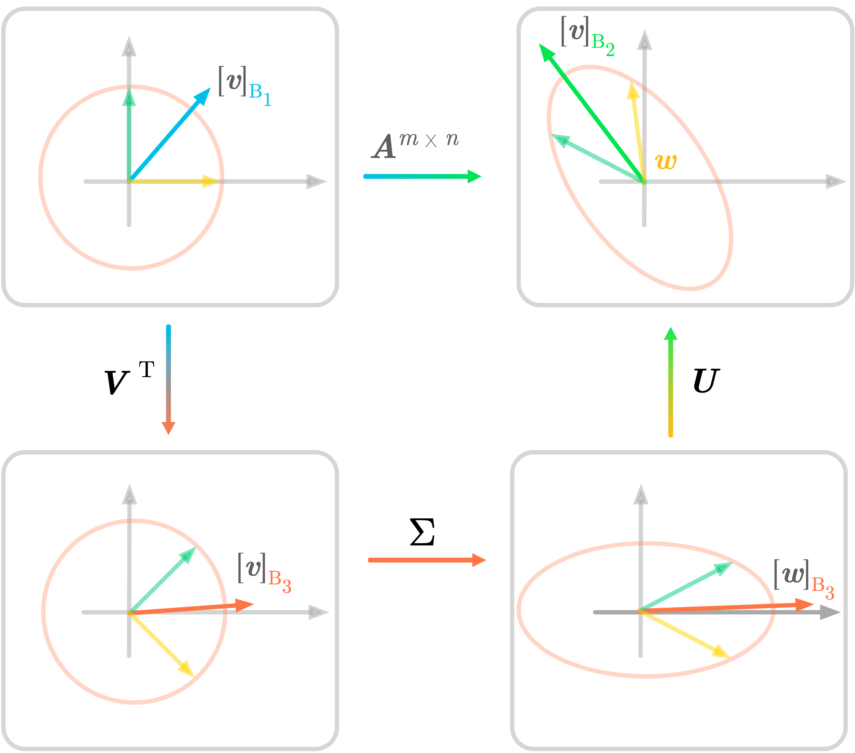
SVD explains $A x$ (applying matrix $A$ to vector $x$ ) as three sequential transformations:

A x = \underset{3. rotate}{\underset{⏟}{U}} \underset{2. stretch}{\underset{⏟}{Σ}} \underset{1. rotate}{\underset{⏟}{V^{⊤}}} x

Physical Steps, Right-to-Left:

$V^{⊤}$ — Rotate the Input:
Align the incoming vector ( $x$ ) with the "natural input axes" ( $v_{i}$ , the right singular vectors).
$Σ$ — Stretch:
Scale each of the input axes by the singular values ( $σ_{i}$ ). This step changes the lengths of vectors, i.e., the magnitude of stretching or shrinking.
$U$ — Rotate the Output:
Reorient the stretched input vector ( $Σ x$ ), turning it into the "natural output axes" ( $u_{i}$ , the left singular vectors).

Derivation: Where $U$ , $Σ$ , and $V$ Come From

The Trick — Turn a Rectangular Matrix Into a Symmetric One

The problem with a general $m \times n$ matrix $A$ is that it is not square, so it has no eigenvectors of its own. The insight behind SVD is simple: multiply $A$ by its own transpose to manufacture a symmetric, square matrix that does have well-behaved eigenvectors.

There are two ways to do this, and each hands us one half of the decomposition:

A^{⊤} A (size n \times n) A A^{⊤} (size m \times m)

Both are symmetric ( $(A^{⊤} A)^{⊤} = A^{⊤} A$ ) and positive semi-definite, so by the spectral theorem each has real, non-negative eigenvalues and a full set of orthogonal eigenvectors.

Assembling the Three Factors

Start from the claim $A = U Σ V^{⊤}$ and see what $A^{⊤} A$ becomes. Because $U^{⊤} U = I$ (the columns of $U$ are orthonormal):

\begin{aligned} A^{⊤} A & = (U Σ V^{⊤})^{⊤} (U Σ V^{⊤}) \\ = V Σ^{⊤} U^{⊤} U Σ V^{⊤} \\ = V \underset{diagonal}{\underset{⏟}{(Σ^{⊤} Σ)}} V^{⊤} \end{aligned}

Compare this with the eigendecomposition $A^{⊤} A = Q Λ Q^{- 1}$ (and note $Q^{- 1} = Q^{⊤}$ since $Q$ is orthogonal). Term by term:

SVD factor	Comes from	Meaning
$V$ (right singular vectors)	eigenvectors of $A^{⊤} A$	natural axes of the input space
$Σ^{⊤} Σ = Λ$	eigenvalues of $A^{⊤} A$ , so $σ_{i} = \sqrt{λ_{i}}$	how much each axis stretches
$U$ (left singular vectors)	eigenvectors of $A A^{⊤}$ (equivalently $u_{i} = \frac{1}{σ_{i}} A v_{i}$ )	natural axes of the output space

That is the whole derivation. SVD is just two coupled eigendecompositions — one for the input space ( $A^{⊤} A$ ) and one for the output space ( $A A^{⊤}$ ) — stitched together by the singular values.

This is the eigenvector → SVD bridge

The right singular vectors are literally the eigenvectors of $A^{⊤} A$ . So if you already understand eigendecomposition, you already understand SVD — you are just eigendecomposing $A^{⊤} A$ and taking square roots of the eigenvalues.

Worked Example — SVD, Step by Step

Let us decompose:

A = [\begin{matrix} 3 & 0 \\ 4 & 5 \end{matrix}]

Step 1 — Form $A^{⊤} A$

A^{⊤} A = [\begin{matrix} 3 & 4 \\ 0 & 5 \end{matrix}] [\begin{matrix} 3 & 0 \\ 4 & 5 \end{matrix}] = [\begin{matrix} 25 & 20 \\ 20 & 25 \end{matrix}]

Step 2 — Eigenvalues of $A^{⊤} A$ (→ singular values)

Solve $det (A^{⊤} A - λ I) = 0$ :

(25 - λ)^{2} - 20^{2} = 0 ⟹ (25 - λ)^{2} = 400 ⟹ 25 - λ = \pm 20

λ_{1} = 45, λ_{2} = 5

The singular values are the square roots:

σ_{1} = \sqrt{45} = 3 \sqrt{5} \approx 6.708, σ_{2} = \sqrt{5} \approx 2.236

Sanity check: the product of singular values equals $| det A |$ . Here $σ_{1} σ_{2} = \sqrt{45} \cdot \sqrt{5} = \sqrt{225} = 15$ , and $| det A | = | 3 \cdot 5 - 0 \cdot 4 | = 15$ ✓

Step 3 — Right singular vectors $V$ (eigenvectors of $A^{⊤} A$ )

For $λ_{1} = 45$ : solve $(A^{⊤} A - 45 I) v = 0$ :

[\begin{matrix} - 20 & 20 \\ 20 & - 20 \end{matrix}] v = 0 \Rightarrow x = y \Rightarrow v_{1} = \frac{1}{\sqrt{2}} [\begin{matrix} 1 \\ 1 \end{matrix}]

For $λ_{2} = 5$ : solve $(A^{⊤} A - 5 I) v = 0$ :

[\begin{matrix} 20 & 20 \\ 20 & 20 \end{matrix}] v = 0 \Rightarrow x = - y \Rightarrow v_{2} = \frac{1}{\sqrt{2}} [\begin{matrix} 1 \\ - 1 \end{matrix}]

V = \frac{1}{\sqrt{2}} [\begin{matrix} 1 & 1 \\ 1 & - 1 \end{matrix}]

Step 4 — Left singular vectors $U$ (via $u_{i} = \frac{1}{σ_{i}} A v_{i}$ )

u_{1} = \frac{1}{σ_{1}} A v_{1} = \frac{1}{3 \sqrt{5}} [\begin{matrix} 3 & 0 \\ 4 & 5 \end{matrix}] \frac{1}{\sqrt{2}} [\begin{matrix} 1 \\ 1 \end{matrix}] = \frac{1}{3 \sqrt{10}} [\begin{matrix} 3 \\ 9 \end{matrix}] = \frac{1}{\sqrt{10}} [\begin{matrix} 1 \\ 3 \end{matrix}]

u_{2} = \frac{1}{σ_{2}} A v_{2} = \frac{1}{\sqrt{5}} [\begin{matrix} 3 & 0 \\ 4 & 5 \end{matrix}] \frac{1}{\sqrt{2}} [\begin{matrix} 1 \\ - 1 \end{matrix}] = \frac{1}{\sqrt{10}} [\begin{matrix} 3 \\ - 1 \end{matrix}]

U = \frac{1}{\sqrt{10}} [\begin{matrix} 1 & 3 \\ 3 & - 1 \end{matrix}]

Step 5 — Assemble and verify $A = U Σ V^{⊤}$

A = \underset{U}{\underset{⏟}{\frac{1}{\sqrt{10}} [\begin{matrix} 1 & 3 \\ 3 & - 1 \end{matrix}]}} \underset{Σ}{\underset{⏟}{[\begin{matrix} 3 \sqrt{5} & 0 \\ 0 & \sqrt{5} \end{matrix}]}} \underset{V^{⊤}}{\underset{⏟}{\frac{1}{\sqrt{2}} [\begin{matrix} 1 & 1 \\ 1 & - 1 \end{matrix}]}}

Multiplying $U Σ$ first, then $V^{⊤}$ , reproduces $[\begin{matrix} 3 & 0 \\ 4 & 5 \end{matrix}] = A$ ✓. The matrix $A$ takes the unit circle and stretches it into an ellipse with semi-axes $6.708$ and $2.236$ .

Applications & Practical Use

Low-Rank Approximation — The Superpower

Because the singular values are sorted $σ_{1} \geq σ_{2} \geq \dots$ , the first few terms of the SVD carry most of the "energy" of the matrix. We can throw away the rest and keep an excellent approximation. Writing SVD as a sum of rank-1 pieces:

A = \sum_{i = 1}^{r} σ_{i} u_{i} v_{i}^{⊤} \approx \sum_{i = 1}^{k} σ_{i} u_{i} v_{i}^{⊤} (k ≪ r)

Keeping only the top $k$ terms gives the best possible rank- $k$ approximation of $A$ (the Eckart–Young theorem). This single idea powers most SVD applications:

Application	How SVD is used
Dimensionality reduction / PCA	Keep the top- $k$ right singular vectors as the new feature axes
Image compression	Store only the top- $k$ singular values/vectors instead of every pixel
Recommender systems	Factor the sparse user–item matrix; latent factors = singular vectors
Latent Semantic Analysis (NLP)	SVD of a term–document matrix reveals hidden topics
Noise reduction / denoising	Small singular values usually correspond to noise — drop them
Solving least-squares / pseudo-inverse	The Moore–Penrose pseudo-inverse is built directly from the SVD

Quick intuition — image compression

A grayscale image is just a matrix of pixel intensities. Its SVD often has a handful of large singular values and a long tail of tiny ones. Reconstructing with only the top ~50 singular values (out of, say, 1000) can look nearly identical to the eye while storing a fraction of the numbers — that is lossy compression, powered entirely by dropping small $σ_{i}$ .

When to Reach for SVD?

You have a rectangular matrix (more samples than features, or vice versa).
You need numerical stability and can't afford the precision loss of forming a covariance matrix.
You want a best low-rank approximation (compression, denoising, latent factors).
You are implementing PCA and want the robust route.

Common Questions & Answers

Q1. How PCA and SVD Differ

They compute the same directions, but they are not interchangeable in practice. The differences matter.

Aspect	PCA	SVD
What it operates on	The covariance matrix $C = \frac{1}{n - 1} X^{⊤} X$	The data matrix $X$ directly
Requires centering?	Yes — data must be mean-centered (and usually standardized)	No — works on any matrix; centering is optional and only needed to make it equal PCA
Matrix shape	Needs a square, symmetric covariance matrix	Works on any $m \times n$ matrix
Numerical stability	Forming $X^{⊤} X$ squares the condition number → precision loss	Operates on $X$ → far more stable and accurate
Output	Eigenvectors (PCs) + eigenvalues (variance)	$U$ , $Σ$ , $V$ — richer: gives both row-space and column-space axes
Scope	A specific application (variance-maximizing projection)	A general matrix factorization — PCA is one of its many uses

The punchline

PCA is SVD in disguise. The principal components ( $W$ ) are exactly the right singular vectors ( $V$ ), and the PCA eigenvalues are the singular values squared (scaled by $n - 1$ ). Running SVD on centered data gives you PCA — without ever building the covariance matrix.

Practical takeaway

Real libraries (scikit-learn's PCA, NumPy, etc.) implement PCA using SVD under the hood, precisely because forming the covariance matrix throws away numerical precision. So even when you call PCA, SVD is usually doing the work.

One more distinction: eigenvalues vs. singular values

This is worth repeating because it trips people up. Eigenvalues can be negative or complex (they describe how a square matrix scales a direction, sign included). Singular values are always $\geq 0$ (they are lengths of ellipse axes). See the "Common Pitfall" callout above.

Q2. How SVD Orders Importance?

In Singular Value Decomposition ( $A = U Σ V^{T}$ ), the "importance" of each singular vector is directly dictated by its corresponding singular value ( $σ_{i}$ ).

By mathematical convention, the singular values in the diagonal matrix $Σ$ are always sorted in descending order:

σ_{1} \geq σ_{2} \geq σ_{3} \geq \dots \geq σ_{r} > 0

Because the matrices $U$ (left singular vectors) and $V$ (right singular vectors) are ordered to match the columns and rows of $Σ$ , they automatically inherit this exact same hierarchy:

Q3. Why Are Singular Values ( $σ$ ) Never Negative?

There are two primary ways to understand why $σ \geq 0$ : geometrically (as a physical length) and algebraically (through the eigenvalues of a symmetric matrix).

1. Geometrically: Scaling Factors Cannot Be Negative

Singular values represent the lengths of the principal semi-axes of the hyper-ellipsoid mapped by the matrix.

Just as the length, width, or height of a physical box cannot be negative, the stretching factor ( $σ$ ) along a singular vector cannot be negative.
If a transformation reverses the direction of a vector, that directional flip is handled entirely by a sign change in the corresponding left singular vector ( $u_{i}$ ), never by making the singular value ( $σ_{i}$ ) negative.

2. Algebraically: They Are Square Roots of Positive Eigenvalues

The right singular vectors $v_{i}$ are the eigenvectors of the matrix $A^{T} A$ . Let's look at the eigenvalue equation for $A^{T} A$ :

(A^{T} A) v_{i} ​ = λ_{i} ​ v_{i}

Because $A^{T} A$ is a symmetric, positive semi-definite matrix, its eigenvalues $λ_{i}$ are mathematically guaranteed to be non-negative ( $λ_{i} \geq 0$ ).

The singular values $σ_{i}$ are defined as the square roots of these eigenvalues:

​ σ_{i} ​ = \sqrt{λ_{i} ​}

Since we always take the principal (positive) square root of a non-negative number $λ_{i}$ , $σ_{i}$ is strictly non-negative ( $σ_{i} \geq 0$ ).

Q4. What is "Thin" or "Truncated" or "Reduced" SVD?

In practical computer science and data science applications (like PCA or image compression), we often use a variation called Thin SVD (or Reduced SVD).

If $A$ is a tall matrix ( $m > n$ ), we don't actually need all $m$ left singular vectors because many of them will just multiply by zeros in $Σ$ . In Thin SVD:

$U$ is truncated to size $m \times n$ (which is not square).
$Σ$ becomes a square $n \times n$ diagonal matrix.
$V^{T}$ remains square at $n \times n$ .

Singular Value Decomposition (SVD)

Understanding Singular Value Decomposition (SVD)

1. Left Singular Vectors (U from AAT)

2. Right Singular Vectors (V from A⊤A)

3. Singular Values (Σ)

4. Mutual Properties of SVD (Orthonormal Bases & Vector Spaces)

Geometric Interpretation of SVD

Derivation: Where U, Σ, and V Come From

Worked Example — SVD, Step by Step

Applications & Practical Use

Low-Rank Approximation — The Superpower

When to Reach for SVD?

Common Questions & Answers

Q1. How PCA and SVD Differ

Q2. How SVD Orders Importance?

Q3. Why Are Singular Values (σ) Never Negative?

Q4. What is "Thin" or "Truncated" or "Reduced" SVD?

1. Left Singular Vectors ( $U$ from $A A^{T}$ )

2. Right Singular Vectors ( $V$ from $A^{⊤} A$ )

3. Singular Values ( $Σ$ )

Derivation: Where $U$ , $Σ$ , and $V$ Come From

Q3. Why Are Singular Values ( $σ$ ) Never Negative?