Eigenvectors & Eigenvalues for Machine Learning

Big Picture

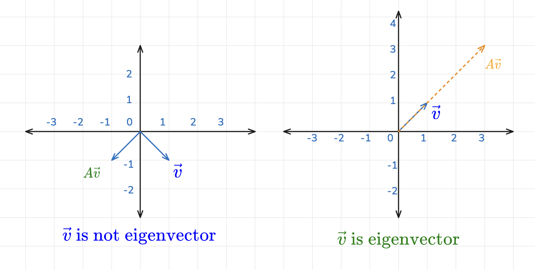
A matrix is a transformation — it takes vectors and moves, rotates, stretches, or squishes them. For almost every vector, a matrix changes its direction. But a special few vectors keep their direction and only get stretched or shrunk. Those special vectors are eigenvectors, and the amount each is stretched is its eigenvalue.

Eigenvectors reveal the "natural axes" of a transformation — the hidden structure inside a matrix. This is exactly what many ML algorithms exploit: PCA finds the directions of maximum variance, spectral clustering finds community structure, and PageRank finds the "importance" vector of a web graph.

Part I — The Idea

1. Prerequisite: A Matrix is a Transformation

Before eigenvectors make sense, recall what multiplying a vector by a matrix does. A square matrix $A$ takes an input vector $v$ and produces an output vector $A v$ — it transforms the vector.

Take the matrix $A = [\begin{matrix} 2 & 0 \\ 0 & 1 \end{matrix}]$ (it doubles the $x$ -coordinate, leaves $y$ alone):

A [\begin{matrix} 1 \\ 1 \end{matrix}] = [\begin{matrix} 2 \\ 1 \end{matrix}] A [\begin{matrix} 1 \\ 0 \end{matrix}] = [\begin{matrix} 2 \\ 0 \end{matrix}] A [\begin{matrix} 0 \\ 1 \end{matrix}] = [\begin{matrix} 0 \\ 1 \end{matrix}]

Notice something:

The vector $[\begin{matrix} 1 \\ 1 \end{matrix}]$ changed direction (it now tilts more toward the $x$ -axis).
The vector $[\begin{matrix} 1 \\ 0 \end{matrix}]$ kept its direction and only got twice as long.
The vector $[\begin{matrix} 0 \\ 1 \end{matrix}]$ kept its direction and its length unchanged.

Those last two vectors — the ones that don't rotate — are the eigenvectors of $A$ . Everything below is about finding them.

2. What Are Eigenvectors and Eigenvalues?

Eigenvectors are nonzero vector that are associated with a matrix such that when the matrix multiplies the eigenvector, the resulting vector is a scalar multiple of the same eigenvector.

\begin{array}{r} \underset{matrix}{\underset{⏟}{A}} \underset{eigenvector}{\underset{⏟}{\vec{v}}} = \underset{eigenvalue}{\underset{⏟}{λ}} \underset{eigenvector}{\underset{⏟}{\vec{v}}} \end{array}

To say that $A \vec{v} = λ \vec{v}$ means that $A \vec{v}$ and $λ \vec{v}$ are collinear with the origin i.e $A \vec{v}$ and $\vec{v}$ lie on the same line through the origin.

Eigenvectors are the directions that remain unchanged during a transformation, even if they get longer or shorter.
Eigenvalues are the numbers that indicate how much the eigenvector stretches or shrinks during that transformation.
Eigenvectors are also called characteristic vectors and can only be found for square matrices ( $n \times n$ ).

The One Equation That Defines Everything

$A \vec{v} = λ \vec{v}$

$A$ — a square matrix (the transformation)
$\vec{v}$ — the eigenvector (a non-zero vector whose direction is preserved)
$λ$ (lambda) — the eigenvalue (the scalar stretch/shrink factor)

In words: "Transforming $\vec{v}$ with $A$ gives the same result as simply scaling $\vec{v}$ by the number $λ$ ."

The word "eigen"

"Eigen" is German for "own" or "characteristic." An eigenvector is a vector that a matrix treats as its "own" special direction — it belongs to the transformation.

2.1 Reading the Eigenvalue

The eigenvalue $λ$ tells you exactly what happens to the eigenvector's length and orientation:

Eigenvalue $λ$	Effect on the eigenvector
$λ > 1$	Stretched — same direction, longer
$0 < λ < 1$	Shrunk — same direction, shorter
$λ = 1$	Unchanged — the vector is completely fixed
$λ = 0$	Collapsed to zero — the direction is in the matrix's null space
$λ < 0$	Flipped — reversed direction, then scaled by $\| λ \|$

3. Geometric Intuition

Imagine placing a rubber sheet with an arrow grid on it and then stretching the sheet with your hands (the "stretch" is the matrix $A$ ).

Most arrows get twisted to point in a new direction.
A few special arrows still point the exact same way as before — they only got longer or shorter. Those are the eigenvectors.
How much longer/shorter each of those special arrows became is its eigenvalue.

Analogy: A Spinning Globe

Spin a globe. Every city on the surface moves — except the two points on the axis of rotation (the North and South Poles). The axis of rotation is the eigenvector: the one direction that doesn't move under the "rotation transformation." For a pure rotation the eigenvalue along that axis is $λ = 1$ (points on the axis don't even change length).

Analogy: Squishing Dough

Press a ball of dough flat between two boards. It spreads wide (a big stretch, large $λ$ ) in the horizontal directions and gets thin (a big shrink, small $λ$ ) vertically. The horizontal and vertical directions are the eigenvectors; the amount of spread/squish in each is the eigenvalue. The eigenvectors are the "natural axes" along which the transformation acts most simply.

Part II — Computing Them

4. The Characteristic Equation

We want non-zero eigenvectors $\vec{v}$

\begin{matrix} (1) & A \vec{v} = λ \vec{v} \end{matrix}

Rearranging:

\begin{array}{r} A \vec{v} - λ \vec{v} = 0 \\ (2) & (A - λ I) \vec{v} = 0 \end{array}

Here $I$ is the identity matrix (we insert it so we can subtract $λ$ (which is scalar), from a matrix).
It has a non-zero solution $\vec{v}$ only if the matrix $(A - λ I)$ is singular — i.e., its determinant is zero:

det (A - λ I) = 0

This is the characteristic equation. Solving it gives the eigenvalues $λ$ ; plugging each $λ$ back into $(A - λ I) v = 0$ gives the eigenvectors.

Why the determinant must be zero?

If $(A - λ I)$ were invertible (non-zero), the only solution would be $v = 0$ — the trivial one we don't want (the zero vector is never an eigenvector). A non-trivial solution exists precisely when the matrix squishes some direction down to nothing, which is exactly what $det = 0$ means.

The Recipe (3 Steps)

Eigenvalues: Solve $det (A - λ I) = 0$ for $λ$ .
Eigenvectors: For each $λ$ , solve $(A - λ I) v = 0$ for $v$ .
(Optional) Normalize: Scale each eigenvector to length 1 (common in ML).

5. Worked Example — 2×2 Matrix (Step by Step)

Let's find the eigenvalues and eigenvectors of:

A = [\begin{matrix} 4 & 1 \\ 2 & 3 \end{matrix}]

Step 1 — Form $A - λ I$

A - λ I = [\begin{matrix} 4 & 1 \\ 2 & 3 \end{matrix}] - [\begin{matrix} λ & 0 \\ 0 & λ \end{matrix}] = [\begin{matrix} 4 - λ & 1 \\ 2 & 3 - λ \end{matrix}]

Step 2 — Set the determinant to zero (characteristic equation)

For a $2 \times 2$ matrix $[\begin{matrix} a & b \\ c & d \end{matrix}]$ , the determinant is $a d - b c$ :

det (A - λ I) = (4 - λ) (3 - λ) - (1) (2) = 0

Expand:

12 - 4 λ - 3 λ + λ^{2} - 2 = 0 ⟹ λ^{2} - 7 λ + 10 = 0

Step 3 — Solve for the eigenvalues

Factor the quadratic:

(λ - 5) (λ - 2) = 0 ⟹ λ_{1} = 5, λ_{2} = 2

Step 4 — Find the eigenvector for $λ_{1} = 5$

Substitute $λ = 5$ into $(A - λ I) v = 0$ :

[\begin{matrix} 4 - 5 & 1 \\ 2 & 3 - 5 \end{matrix}] [\begin{matrix} x \\ y \end{matrix}] = [\begin{matrix} - 1 & 1 \\ 2 & - 2 \end{matrix}] [\begin{matrix} x \\ y \end{matrix}] = [\begin{matrix} 0 \\ 0 \end{matrix}]

Both rows give the same equation: $- x + y = 0 \Rightarrow y = x$ . So any vector along $[\begin{matrix} 1 \\ 1 \end{matrix}]$ works:

v_{1} = [\begin{matrix} 1 \\ 1 \end{matrix}]

Step 5 — Find the eigenvector for $λ_{2} = 2$

Substitute $λ = 2$ :

[\begin{matrix} 4 - 2 & 1 \\ 2 & 3 - 2 \end{matrix}] [\begin{matrix} x \\ y \end{matrix}] = [\begin{matrix} 2 & 1 \\ 2 & 1 \end{matrix}] [\begin{matrix} x \\ y \end{matrix}] = [\begin{matrix} 0 \\ 0 \end{matrix}]

This gives $2 x + y = 0 \Rightarrow y = - 2 x$ . So an eigenvector is:

v_{2} = [\begin{matrix} 1 \\ - 2 \end{matrix}]

Step 6 — Verify $A v = λ v$

A v_{1} = [\begin{matrix} 4 & 1 \\ 2 & 3 \end{matrix}] [\begin{matrix} 1 \\ 1 \end{matrix}] = [\begin{matrix} 5 \\ 5 \end{matrix}] = 5 [\begin{matrix} 1 \\ 1 \end{matrix}] = λ_{1} v_{1} ✓

A v_{2} = [\begin{matrix} 4 & 1 \\ 2 & 3 \end{matrix}] [\begin{matrix} 1 \\ - 2 \end{matrix}] = [\begin{matrix} 2 \\ - 4 \end{matrix}] = 2 [\begin{matrix} 1 \\ - 2 \end{matrix}] = λ_{2} v_{2} ✓

Both check out. The matrix $A$ stretches the $[\begin{matrix} 1 \\ 1 \end{matrix}]$ direction by 5× and the $[\begin{matrix} 1 \\ - 2 \end{matrix}]$ direction by 2×.

6. Handy Shortcuts & Properties

For an $n \times n$ matrix there are (counting multiplicity) $n$ eigenvalues. Two identities are great for checking your work:

Property	Rule	Check on the example ( $λ = 5, 2$ )
Sum of eigenvalues	$= trace (A)$ (sum of the diagonal)	$5 + 2 = 7 = 4 + 3 ✓$
Product of eigenvalues	$= det (A)$	$5 \times 2 = 10 = (4) (3) - (1) (2) ✓$

Other useful facts:

Eigenvectors are not unique — any non-zero scalar multiple of an eigenvector is also an eigenvector (same direction). This is why we often normalize to length 1.
Symmetric matrices ( $A = A^{⊤}$ ) always have real eigenvalues and orthogonal (perpendicular) eigenvectors. Covariance matrices are symmetric — which is what makes PCA work so cleanly.
If any eigenvalue is $0$ , the matrix is singular (non-invertible).

Part III — Eigendecomposition

7. Breaking a Matrix into Its Eigen-Parts

If an $n \times n$ matrix $A$ has $n$ independent eigenvectors, we can factor it into its eigenvalues and eigenvectors. This is eigendecomposition (or diagonalization):

A = Q Λ Q^{- 1}

Where:

$Q$ — a matrix whose columns are the eigenvectors of $A$ .
$Λ$ — a diagonal matrix with the eigenvalues on the diagonal.
$Q^{- 1}$ — the inverse of $Q$ .

Intuition: this splits the transformation into three simple stages — rotate into the eigenvector coordinate system ( $Q^{- 1}$ ), stretch along each axis ( $Λ$ ), then rotate back ( $Q$ ). In the eigenvector coordinate system, the complicated matrix $A$ becomes a simple set of independent stretches.

From the worked example in §5, we found:

λ_{1} = 5, v_{1} = [\begin{matrix} 1 \\ 1 \end{matrix}] λ_{2} = 2, v_{2} = [\begin{matrix} 1 \\ - 2 \end{matrix}]

Step 1 — Build $Q$ (columns = eigenvectors):

Q = [\begin{matrix} 1 & 1 \\ 1 & - 2 \end{matrix}]

Step 2 — Build $Λ$ (eigenvalues on diagonal):

Λ = [\begin{matrix} 5 & 0 \\ 0 & 2 \end{matrix}]

Step 3 — Compute $Q^{- 1}$ :
For a $2 \times 2$ matrix $[\begin{matrix} a & b \\ c & d \end{matrix}]$ , the inverse is $\frac{1}{a d - b c} [\begin{matrix} d & - b \\ - c & a \end{matrix}]$ .

det (Q) = (1) (- 2) - (1) (1) = - 3

Q^{- 1} = \frac{1}{- 3} [\begin{matrix} - 2 & - 1 \\ - 1 & 1 \end{matrix}] = [\begin{matrix} \frac{2}{3} & \frac{1}{3} \\ \frac{1}{3} & - \frac{1}{3} \end{matrix}]

Step 4 — Verify $Q Λ Q^{- 1} = A$ :

Q Λ = [\begin{matrix} 1 & 1 \\ 1 & - 2 \end{matrix}] [\begin{matrix} 5 & 0 \\ 0 & 2 \end{matrix}] = [\begin{matrix} 5 & 2 \\ 5 & - 4 \end{matrix}]

Q Λ Q^{- 1} = [\begin{matrix} 5 & 2 \\ 5 & - 4 \end{matrix}] [\begin{matrix} \frac{2}{3} & \frac{1}{3} \\ \frac{1}{3} & - \frac{1}{3} \end{matrix}] = [\begin{matrix} \frac{10}{3} + \frac{2}{3} & \frac{5}{3} - \frac{2}{3} \\ \frac{10}{3} - \frac{4}{3} & \frac{5}{3} + \frac{4}{3} \end{matrix}] = [\begin{matrix} 4 & 1 \\ 2 & 3 \end{matrix}] = A ✓

Bonus — Computing $A^{3}$ the easy way:

A^{3} = Q Λ^{3} Q^{- 1}, Λ^{3} = [\begin{matrix} 5^{3} & 0 \\ 0 & 2^{3} \end{matrix}] = [\begin{matrix} 125 & 0 \\ 0 & 8 \end{matrix}]

No repeated matrix multiplication needed — just raise each eigenvalue to the power.

Why this is powerful

Once $A = Q Λ Q^{- 1}$ , computing powers becomes trivial: $A^{k} = Q Λ^{k} Q^{- 1}$ , and $Λ^{k}$ is just each eigenvalue raised to the $k$ . This is the backbone of analyzing repeated/iterative processes (Markov chains, PageRank, the stability of dynamical systems).

Related: Singular Value Decomposition (SVD)

Eigendecomposition only works for square matrices. SVD generalizes the idea to any $m \times n$ matrix by decomposing it into $A = U Σ V^{⊤}$ , where the "singular values" in $Σ$ play the role of eigenvalue magnitudes. SVD underlies many ML tools (recommender systems, latent semantic analysis, and a numerically stable way to compute PCA).

Part IV — Applications in Machine Learning

Eigenvectors and eigenvalues are not an abstract curiosity — they power some of the most-used algorithms in ML. The recurring theme: find the directions that matter most.

8. Principal Component Analysis (PCA) — The Flagship Use

This is the single most important application. PCA reduces the number of features while keeping as much information (variance) as possible.

The connection:

Compute the covariance matrix of the data — a symmetric matrix describing how features vary together.
Find its eigenvectors and eigenvalues.
The eigenvectors are the principal components — the directions of maximum variance in the data.
The eigenvalue of each eigenvector = the amount of variance captured along that direction.
Keep the eigenvectors with the largest eigenvalues (most information) and drop the rest → dimensionality reduction.

Intuition

Picture a stretched, cigar-shaped cloud of 2-D data points. The long axis of the cloud is the eigenvector with the largest eigenvalue — the direction where the data varies most. Projecting every point onto just that one axis keeps most of the information while collapsing 2-D down to 1-D. That is PCA in a nutshell.

The eigenvalues also tell you how much you can safely discard: the explained variance ratio of a component is its eigenvalue divided by the sum of all eigenvalues.

Variance explained by component i = \frac{λ_{i}}{λ_{1} + λ_{2} + \dots + λ_{n}}

See the full step-by-step eigen-decomposition worked example in the PCA note.

9. Other Key Applications

Application	Role of Eigenvectors / Eigenvalues
Covariance & correlation analysis	Eigenvectors of the covariance matrix expose the axes of greatest spread; eigenvalues quantify the spread — the foundation of PCA and whitening.
Spectral Clustering	Build a graph of the data, form its Laplacian matrix, and use its smallest eigenvectors to embed points so clusters become linearly separable — great for non-spherical clusters that k-means fails on.
PageRank (Google)	The ranking of web pages is the dominant eigenvector of the web's link matrix (eigenvalue $λ = 1$ ) — the steady-state "importance" of each page.
Recommender Systems	Matrix factorization (via SVD) uncovers latent factors — the eigen-directions of the user–item matrix — to predict missing ratings.
Image Compression	Keeping only the top eigenvectors (largest eigenvalues) of an image reconstructs it with far less data (e.g., "eigenfaces" for face recognition).
Deep Learning stability	Eigenvalues of the Hessian describe the curvature of the loss surface (conditioning, saddle points); eigenvalues of weight matrices relate to exploding/vanishing gradients.
Dynamical systems / RNNs	The largest-magnitude eigenvalue of a transition/weight matrix governs whether repeated application makes signals grow, shrink, or stay stable.

10. Quick ML Example — Which Direction Carries the Signal?

Suppose after standardizing a small 2-feature dataset (e.g., height and weight) we compute the covariance matrix:

C = [\begin{matrix} 1.0 & 0.8 \\ 0.8 & 1.0 \end{matrix}]

Its eigenvalues are $λ_{1} = 1.8$ and $λ_{2} = 0.2$ (using $λ = 1 \pm 0.8$ for this symmetric form), with eigenvectors:

v_{1} = [\begin{matrix} 1 \\ 1 \end{matrix}] (the 45^{\circ} "size" axis), v_{2} = [\begin{matrix} 1 \\ - 1 \end{matrix}] (the "shape" axis)

Interpretation: $v_{1}$ (large eigenvalue $1.8$ ) captures $\frac{1.8}{1.8 + 0.2} = 90 %$ of the variance — tall people tend to be heavier, so most of the information lives along this combined "overall size" direction. We could keep only the $v_{1}$ component and describe each person with a single number while losing just 10% of the variance. That is PCA reducing 2 features to 1.

11. Summary

Concept	Meaning	Formula
Matrix as transformation	A square matrix moves/stretches vectors	$A v$
Eigenvector $v$	Direction unchanged by the transformation	$A v = λ v$
Eigenvalue $λ$	How much the eigenvector is stretched/shrunk	$A v = λ v$
Characteristic equation	How we solve for eigenvalues	$det (A - λ I) = 0$
Trace check	Sum of eigenvalues = diagonal sum	$\sum λ_{i} = trace (A)$
Determinant check	Product of eigenvalues	$\prod λ_{i} = det (A)$
Eigendecomposition	Factoring a matrix into eigen-parts	$A = Q Λ Q^{- 1}$
PCA link	Eigenvectors of covariance = principal components	$variance \propto λ_{i}$

The Big Picture

A matrix transforms vectors — usually changing their direction.
Eigenvectors are the special directions that don't rotate; eigenvalues say how much they stretch.
We find them by solving $det (A - λ I) = 0$ , then back-substituting.
Eigendecomposition ( $A = Q Λ Q^{- 1}$ ) reveals the simple stretches hiding inside any diagonalizable matrix.
In ML they find the directions that matter — maximum-variance axes in PCA, community structure in spectral clustering, and importance in PageRank.

The core takeaway: Eigenvectors are the natural axes of a transformation, and eigenvalues measure their importance. Whenever an ML method needs to find "the directions that matter most," eigenvectors and eigenvalues are doing the work.

12. Questions and Answers

What does the equation $A v = λ v$ mean in plain words?
$A n s .$ Transforming the vector $v$ with the matrix $A$ produces the same result as simply scaling $v$ by the number $λ$ — i.e., $v$ 's direction is unchanged and it is only stretched/shrunk by $λ$ .
Can a non-square matrix have eigenvectors?
$A n s .$ No. Eigenvectors/eigenvalues are defined only for square ( $n \times n$ ) matrices. For rectangular matrices we use the closely related SVD (singular values) instead.
Why do symmetric matrices (like covariance matrices) matter so much in ML?
$A n s .$ Symmetric matrices are guaranteed to have real eigenvalues and orthogonal (perpendicular) eigenvectors. Because a covariance matrix is symmetric, its eigenvectors form a clean set of perpendicular axes — exactly what PCA needs to define uncorrelated principal components.
In PCA, what do a large vs. small eigenvalue tell you?
$A n s .$ A large eigenvalue means its eigenvector (principal component) captures a lot of the data's variance — keep it. A small eigenvalue means that direction carries little information — it can be dropped to reduce dimensionality with minimal loss.
A $2 \times 2$ matrix has $trace = 6$ and $det = 8$ . What are its eigenvalues?
$A n s .$ The eigenvalues satisfy $λ_{1} + λ_{2} = 6$ and $λ_{1} λ_{2} = 8$ , giving $λ = 4$ and $λ = 2$ .