R-Squared (The "Accuracy Score" of your Model)

What is R-Squared?

R-Squared ( $R^{2}$ ), also called the Coefficient of Determination, is a single number between 0 and 1 that tells you: "What percentage of the variation in my outcome ( $Y$ ) is explained by my predictor(s) ( $X$ )?"

🎯 Part 1: The Setup - What Are We Trying to Measure?

Imagine you are trying to predict something, like how well you'll do on a test based on how many hours you studied. R-Squared is the grade we give to our prediction "rule" to see how much of the story it actually tells.

$X$ (Independent Variable): Hours studied
$Y$ (Dependent Variable): Exam score

You collect data from 50 students and fit a regression line:

\hat{y} = m x + b

Where:

$m$ = slope = $r \cdot \frac{σ_{y}}{σ_{x}}$
$b$ = intercept = $\bar{y} - m \bar{x}$
$\hat{y}$ = predicted score

The Central Question: How well does this line predict the actual scores?

This is exactly what R-squared measures.

🧩 Part 2: The Intuition - Two Competing Model

Think of it as a competition between two models:

★ Model 1: "The Lazy Guesser" (The Mean)

Predicting everything using just the average ( $μ_{y}$ ). This is our baseline.
Any "mistake" here is called Total Variation (SST) .

★ Model 2: "The Smart Predictor" (The Regression Line)**

Predicting using our $(\hat{y} = m x + b)$ formula.
Any "mistake" left over here is called Unexplained Variation (SSE).

What does R-squared asks?

"How much did we reduce our errors by being smart instead of lazy?"

🧱 Part 3: The Building Blocks

★ Block 1: Understand mean score

Imagine ignoring study hours completely. The best guess for any student’s score would be:

μ_{y} = \frac{\sum_{i = 1}^{n} x_{i}}{n} \dots where x_{i} is score of n students.

This is called as the mean score $μ_{y}$

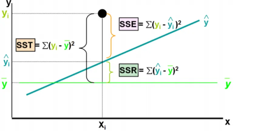
★ Block 2: The "Baseline" Model ➛ SST (Total Sum of Squares)

This measures total variability if you ignored $X$ completely and just guessed $μ_{y}$ for everyone.

Concept: Imagine you had no model at all; you would simply guess the average value $μ_{y}$ for every prediction. SST represents the total error of those "average" guesses.

\begin{array}{r} S S T = \sum_{i = 1}^{n} (y_{i} - μ_{y})^{2} \dots y_{i} is the actual value of the i^{t h} observation. \end{array}

What it represents:

The total "mystery" or uncertainty in your data
How spread out the scores are from the mean
The maximum possible error if you had no model

★ Block 3: The "Smart" Model ➛ SSR (Regression Sum of Squares)

This measures how much variability your regression line successfully explained by our model.

Concept: SSR represents how much "better" your regression line is at predicting the data compared to just guessing the average.

The amount of "total mistakes" that our smart line successfully explained. i.e quantifies how much the data points ( $y_{i}$ ), vary around the estimated regression line( $\hat{y_{i}}$ ).

S S E = \sum_{i = 1}^{n} (y_{i} - {\hat{y}}_{i})^{2}

What it represents:

The vertical distance between actual points and your predictions
The "noise" or factors you missed
The unexplained variance

★ Block 4: The "Leftover Mistakes" ➛ SSE (Sum of Squared Errors)

This measures the variability that your model failed to explain (the residuals).

Concept: These are the "residuals." It represents the noise or factors that your features failed to capture.

The "mistakes" that are still there even after using our smart line. i.e quantifies how far the estimated sloped regression line, $\hat{y_{i}}$ , is from the horizontal "no relationship line," the sample mean or $μ_{y}$ .

S S E = \sum_{i = 1}^{n} (y_{i} - {\hat{y}}_{i})^{2}

What it represents:

The vertical distance between actual points and your predictions
The "noise" or factors you missed
The unexplained variance

★ The Golden Equation

These three pieces always follow this relationship:

S S T = S S R + S S E

In words: $$\boxed{\Large \text{Total Variation} = \text{Explained Variation} + \text{Unexplained Variation}}$$

🧮 Part 4: The $R^{2}$ Formula

Now we can define R-squared in two equivalent ways:

★ Method 1: The "Success Ratio"

R^{2} = \frac{Explained Variation}{Total Variation} = \frac{S S R}{S S T}

Interpretation: "What fraction of the total mystery did we solve?"

★ Method 2: The "Mistake Reduction Ratio"

R^{2} = 1 - \frac{Unexplained Variation}{Total Variation} = 1 - \frac{S S E}{S S T}

Interpretation: "If we start with 100% mystery, how much is left over?"

📊📉 Part 5: Visual Summary Table

Component	Formula	What it tells you
$S S T$	$\sum (y_{i} - μ_{y})^{2}$	Total error if you just guessed the average.
$S S R$	$\sum ({\hat{y}}_{i} - μ_{y})^{2}$	How much error you "fixed" by using the model.
$S S E$	$\sum (y_{i} - {\hat{y}}_{i})^{2}$	The error that remains after the model.

🔢 Part 6: Worked Example

★ Given Data:

Total Variation: $S S T = 200$
After fitting your model, the remaining error: $S S E = 50$

★ Calculation:

R^{2} = 1 - \frac{50}{200} = 1 - 0.25 = 0.75

🎓 Part 7: How to Interpret $R^{2}$ Values

The value of $R^{2}$ is always between 0 and 1

If $SSR$ is small, line is a good fit.
If points lie perfectly on a line: $R^{2} = 1$ ➛ The model explains all of the variability in the dependent variable.
If points are completely random: $R^{2} \approx 0$ ➛ The model explains none of the variability in the dependent variable.
$R^{2}$ measures how tightly data hugs the regression line.

R² Value	Meaning	Example Scenario
0.90 - 1.00	Excellent fit	Predicting height from arm length (biology)
0.70 - 0.89	Strong fit	Predicting grades from study hours
0.40 - 0.69	Moderate fit	Predicting happiness from income
0.20 - 0.39	Weak fit	Predicting stock prices from last month
0.00 - 0.19	Very weak	Predicting test scores from shoe size

When is Low R² Acceptable?

Social sciences: Human behavior is complex; $R^{2} = 0.30$ can be useful
Stock markets: Inherently random; even $R^{2} = 0.10$ provides value
Medical research: Many factors affect outcomes; $R^{2} = 0.40$ can save lives

🔗 Part 8: The Connection to Correlation ( $r$ )

For simple linear regression (one $X$ , one $Y$ ):

R^{2} = r^{2}

Where $r$ is the Pearson correlation coefficient between $X$ and $Y$ .

To recover $r$ from $R^{2}$ :

r = \pm \sqrt{R^{2}}

The sign rule:

If slope ( $m$ ) is positive → $r$ is positive
If slope ( $m$ ) is negative → $r$ is negative

⚠️ Part 9: Important Limitations

What R² Does NOT Tell You

It doesn't prove causation: High $R^{2}$ doesn't mean $X$ causes $Y$
It doesn't detect bias: A biased model can have high $R^{2}$
It doesn't validate assumptions: Check residual plots for patterns
It rewards complexity: Adding variables always increases $R^{2}$ (see Adjusted $R^{2}$ below)

🎯 Part 10: The Problem with $R^{2}$ ➛ Enter " $Adjusted R^{2}$ "

⚠️ The Flaw in $R^{2}$

Problem: $R^{2}$ will always increase (or stay the same) when you add more features, even if those features are pure random noise.

Why? The mathematical definition of $R^{2}$ is designed to reward any reduction in $S S E$ , no matter how tiny.

Example of the Problem
You have a model predicting house prices with:

Feature 1: Square footage ( $R^{2} = 0.70$ )
Feature 2: Number of bedrooms ( $R^{2} = 0.75$ ) ✅ Improvement!
Feature 3: Homeowner's favorite color ( $R^{2} = 0.751$ ) 🤔 Wait...

Adding "favorite color" increased $R^{2}$ by 0.001, but it's obviously meaningless!

✅ The Solution: Adjusted $R^{2}$

Adjusted $R^{2}$ penalizes you for adding features that don't pull their weight.

How it works: It only increases if the new feature improves the model's predictive power significantly more than what would be expected by random chance.
The "Drop" Mechanism: If you add a useless feature, the $R^{2}$ might go up by $0.0001$ , but the penalty for adding a new variable will be larger than that tiny gain. The result? The Adjusted $R^{2}$ will actually go down.

🤔 Why Adjusted $R^{2}$ is Better for Your Model?

➛ in case of Multiple linear Regression

A. It Fights Overfitting

Overfitting happens when your model learns the "noise" in your data rather than the actual "signal." By using Adjusted $R^{2}$ , you are visually alerted when your model is getting too complex without adding real value.

B. It Guides Feature Selection

When you are deciding which features to keep:

Add a feature.
The Penalty: It adds a "penalty" for every new feature you add.
If Adjusted $R^{2}$ increases, the feature is adding value.
If Adjusted $R^{2}$ decreases, the feature is likely noise and should be removed.

C. It Accounts for Sample Size ( $n$ )

The formula for Adjusted $R^{2}$ includes the number of data points ( $n$ ). This is crucial because it’s much easier to "fake" a high $R^{2}$ with a small dataset (e.g., 5 points and 4 features) than with a large one. Adjusted $R^{2}$ corrects for this bias.

📝 The Formula:

Adjusted R^{2} = 1 - \frac{S S E / (n - k)}{S S T / (n - 1)}

Where:

$n$ = number of data points
$k$ = number of features (predictors) in your model

📝 Alternative Form:

Adjusted R^{2} = 1 - [(1 - R^{2}) \cdot \frac{n - 1}{n - k}]

📈📉 The "Gap" Test

As a rule of thumb in my lab, I always look at the gap between the two:

Small Gap: Your features are high-quality and relevant.
Large Gap: You have "junk" features that are inflating your $R^{2}$ without providing real predictive power.

★ Visual Comparison:

Scenario	$R^{2}$	Adjusted $R^{2}$	Verdict
3 features, all relevant	0.85	0.84	✅ Good model
10 features, 3 relevant	0.87	0.72	⚠️ Overfitting!
20 features, 2 relevant	0.90	0.55	🚫 Terrible! Too complex

📚 Part 11: Quick Summary

The One-Sentence Summary

R-Squared tells you what percentage of the variation in $Y$ is predictable from $X$ .
Adjusted R-Squared tells you if adding more features is actually helping or just making your model needlessly complex.

Key Formulas at a Glance

Concept	Formula	Alternate Formula
R-Squared	$1 - \frac{S S E}{S S T}$	$\frac{S S R}{S S T}$
Adjusted R-Squared	$1 - \frac{S S E / (n - k)}{S S T / (n - 1)}$	$1 - (1 - R^{2}) \cdot \frac{n - 1}{n - k}$
Correlation	$r = \pm \sqrt{R^{2}}$ (for simple regression)

Final Takeaway

Use $R^{2}$ to see if your model explains a meaningful portion of the variation
Use $Adjusted R^{2}$ when comparing models with different numbers of features
Always visualize residuals to check if your model assumptions are valid
Remember: A high $R^{2}$ doesn't automatically mean a good model—context matters!

R-Squared (The "Accuracy Score" of your Model)

🎯 Part 1: The Setup - What Are We Trying to Measure?

🧩 Part 2: The Intuition - Two Competing Model

★ Model 1: "The Lazy Guesser" (The Mean)

★ Model 2: "The Smart Predictor" (The Regression Line)**

🧱 Part 3: The Building Blocks

★ Block 1: Understand mean score

★ Block 2: The "Baseline" Model ➛ SST (Total Sum of Squares)

★ Block 3: The "Smart" Model ➛ SSR (Regression Sum of Squares)

★ Block 4: The "Leftover Mistakes" ➛ SSE (Sum of Squared Errors)

★ The Golden Equation

🧮 Part 4: The R2 Formula

★ Method 1: The "Success Ratio"

★ Method 2: The "Mistake Reduction Ratio"

📊📉 Part 5: Visual Summary Table

🔢 Part 6: Worked Example

★ Given Data:

★ Calculation:

🎓 Part 7: How to Interpret R2 Values

🔗 Part 8: The Connection to Correlation (r)

⚠️ Part 9: Important Limitations

🎯 Part 10: The Problem with R2 ➛ Enter "AdjustedR2"

⚠️ The Flaw in R2

✅ The Solution: Adjusted R2

🤔 Why Adjusted R2 is Better for Your Model?

A. It Fights Overfitting

B. It Guides Feature Selection

C. It Accounts for Sample Size (n)

📝 The Formula:

📝 Alternative Form:

📈📉 The "Gap" Test

★ Visual Comparison:

📚 Part 11: Quick Summary

🧮 Part 4: The $R^{2}$ Formula

🎓 Part 7: How to Interpret $R^{2}$ Values

🔗 Part 8: The Connection to Correlation ( $r$ )

🎯 Part 10: The Problem with $R^{2}$ ➛ Enter " $Adjusted R^{2}$ "

⚠️ The Flaw in $R^{2}$

✅ The Solution: Adjusted $R^{2}$

🤔 Why Adjusted $R^{2}$ is Better for Your Model?

C. It Accounts for Sample Size ( $n$ )