Stacking with Cross-Validation
Stacking with Cross-Validation (also known as Stacked Generalization) is the traditional and most robust variant of stacking ensemble methods. It uses K-fold cross-validation to generate out-of-fold predictions for training the meta-model, ensuring that every data point in the training set contributes to both base model training and meta-model training. This approach maximizes data efficiency while maintaining proper separation between training and validation to prevent overfitting.
Overview
In cross-validation stacking, the training process leverages the full training dataset through a systematic K-fold cross-validation strategy:
- Training Set: Split into K folds for cross-validation
- Test Set: Reserved exclusively for final evaluation (never seen during training)
- Out-of-Fold Predictions: Generated for the entire training set through CV iterations
The key distinction from blending is that cross-validation stacking uses all training data efficiently—each sample appears in a validation fold exactly once, ensuring the meta-model learns from predictions on the complete training set.
Diagrammatic Workflow
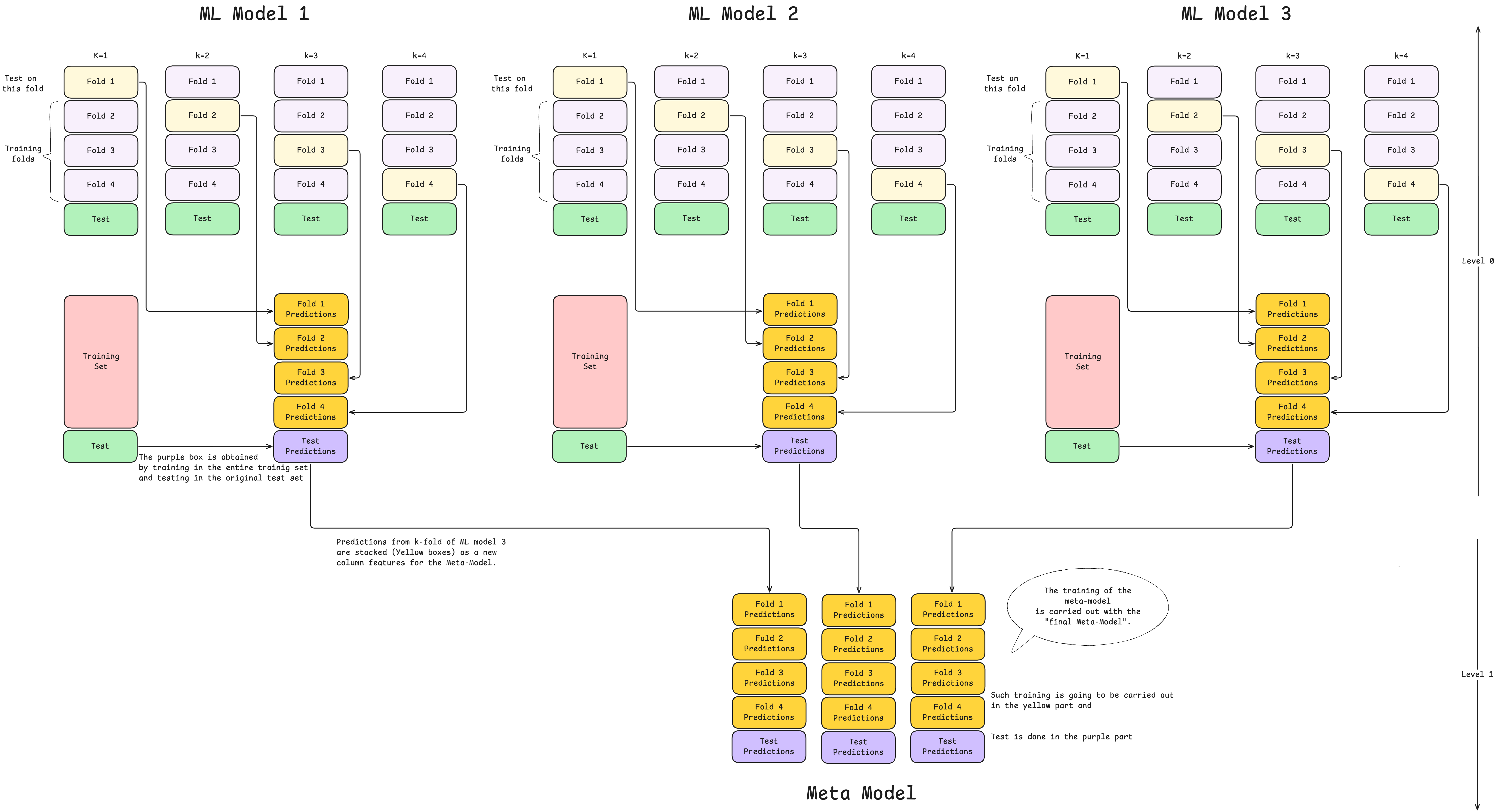
Implementation Process
Level 0: Base Model Development with Cross-Validation
Step 1: Initial Data Partitioning
Split the main dataset into a training set (typically 80%) and a test set (remaining 20%). The test set is held out completely and used only for final performance evaluation.
Step 2: Set Up K-Fold Cross-Validation
Divide the training set into K equal-sized folds (commonly K=5 or K=10). For classification tasks, use 👉 stratified K-fold to maintain class distribution across folds.
Example with K=5:
- Fold 1, 2, 3, 4, 5 (each containing 20% of training data)
Step 3: Train Base Models Using Cross-Validation
For each base model (e.g., Random Forest, XGBoost, Neural Network):
Iteration 1:
- Train on Folds 2, 3, 4, 5 (80% of data)
- Predict on Fold 1 (20% holdout)
Iteration 2:
- Train on Folds 1, 3, 4, 5 (80% of data)
- Predict on Fold 2 (20% holdout)
Continue until Iteration K:
- Train on Folds 1, 2, ..., K-1
- Predict on Fold K
After K iterations, you have out-of-fold predictions for every sample in the training set. Each prediction is truly out-of-sample since it comes from a model that never saw that particular data point during training.
graph TB
    A[Training Data Split into Folds] --> B1[Fold 1 held out]
    A --> B2[Fold 2 held out]
    A --> B3[Fold 3 held out]

    B1 --> C1[Train on other folds]
    B2 --> C2[Train on other folds]
    B3 --> C3[Train on other folds]

    C1 --> D1[Predict on held-out fold]
    C2 --> D2[Predict on held-out fold]
    C3 --> D3[Predict on held-out fold]

    D1 --> E[Combine all OOF predictions]
    D2 --> E
    D3 --> E

    E --> F[Train Meta-Model]

    F --> G[Properly Generalized Model]

    style G fill:#ccffcc
Step 4: Generate Test Set Predictions
For each base model, train a final version on the entire training set (all K folds combined). Then generate predictions on the test set. These will be used later for final evaluation.
Note: Some implementations average predictions from all K fold-trained models instead of training a final model on all data. Both approaches are valid.
Level 1: Meta-Model Training
Step 5: Construct Meta-Training Dataset
Compile the out-of-fold predictions from Step 3 into a new dataset where:
- Each column represents predictions from one base model.
- Each row corresponds to one sample from the original training set
- With 3 base models, you'll have a 3-column dataset with the same number of rows as the training set
Key Advantage: Unlike blending, you now have meta-features for 100% of your training data, not just a holdout subset.
Note: Traditional stacking typically uses only base model predictions as features. However, some advanced implementations (stacking with original features) may concatenate the original features with base predictions to give the meta-model more information.
Step 6: Train the Meta-Model
Fit the meta-model (Level 1 learner) using:
- Input features: Out-of-fold predictions from all base models (Step 5)
- Target values: Original labels from the training set
The meta-model learns the optimal strategy to combine base model predictions. It essentially learns which models to trust under which circumstances and how to weight their contributions.
Common meta-model choices:
- Logistic Regression (for classification)
- Linear Regression (for regression tasks)
- Ridge or Lasso Regression (with regularization)
- Gradient Boosting (for complex combination strategies)
- Neural Networks (for highly non-linear combinations)
Final Phase: Inference and Evaluation
Step 7: Generate Meta-Features for Test Set
Use the test set predictions generated in Step 4 as input to the meta-model. These predictions serve as meta-features, structured identically to the meta-training dataset (one column per base model).
Step 8: Generate Final Predictions
Feed the test set meta-features into the trained meta-model. The meta-model applies its learned combination strategy to produce the final ensemble predictions.
Important: No training occurs at this stage. The meta-model simply uses its learned weights and logic to combine the base model outputs.
Step 9: Evaluate Performance
Compare the final ensemble predictions against the actual test set labels to calculate comprehensive performance metrics:
- Classification: Accuracy, Precision, Recall, F1-score, ROC-AUC
- Regression: RMSE, MAE, R², MAPE
Key Differences: Cross-Validation Stacking vs. Blending
| Aspect | CV Stacking | Blending |
|---|---|---|
| Validation Strategy | K-fold cross-validation | Single holdout split |
| Data Usage | Highly efficient (all data used) | Less efficient (holdout unused by base models) |
| Computation Time | Slower (K training rounds per model) | Faster (single split) |
| Meta-Model Training Data | Full training set (out-of-fold predictions) | Smaller (only holdout set) |
| Robustness | More robust (averaged over K folds) | More variance (single split dependent) |
| Complexity | More complex to implement | Simpler implementation |
Advantages
- Maximum Data Efficiency: Every sample in the training set contributes to both base model training and meta-model training, ensuring no data is wasted
- Robust Out-of-Sample Predictions: Out-of-fold predictions provide genuine unseen predictions for the entire training set, reducing overfitting risk
- Better Generalization: The meta-model trains on a larger and more representative dataset, leading to improved performance
- Reduced Variance: Cross-validation averages out the randomness of any single split, producing more stable and reliable results
- Optimal for Small/Medium Datasets: Makes the most of limited data by using every sample efficiently
Limitations
- Computational Cost: Requires training each base model K times, which can be expensive with large datasets or complex models
- Implementation Complexity: More intricate to code and debug compared to simple holdout validation
- Time-Intensive: Training time increases linearly with K, making it slower for rapid prototyping
- Memory Requirements: Storing K models (or their predictions) requires more memory
- Longer Development Cycle: Iteration and experimentation take longer due to extended training times
When to Use Cross-Validation Stacking
Best suited for:
- Small to medium-sized datasets where data efficiency is paramount
- Projects where maximum predictive performance is the primary goal
- Research settings where computational time is less critical
- Competitions where squeezing out every bit of performance matters
- Scenarios with sufficient computational resources
Avoid when:
- Working with very large datasets where computation time is prohibitive
- Quick prototyping or time-sensitive deployments are required
- Computational resources are severely limited
- Simple blending would provide nearly equivalent performance with much less cost
Practical Tips
-
Choose K Wisely:
- K=5 or K=10 are standard choices
- Smaller K (3-5): Faster, less variance reduction
- Larger K (10-20): Slower, more robust, but diminishing returns beyond K=10
-
Stratified Folds:
- Always use stratified K-fold for classification to maintain class proportions
- Particularly critical for imbalanced datasets
-
Model Diversity:
- Combine different algorithm families (tree-based, linear, neural networks)
- Use models with different strengths and weaknesses
- Diversity drives ensemble performance gains
-
Base Model Quality:
- Tune base models individually before stacking
- Poorly performing base models add noise rather than value
- Balance between model diversity and individual quality
-
Meta-Model Selection:
- Start with simple models (Logistic/Linear Regression)
- Only use complex meta-models if simple ones underperform
- Risk of overfitting increases with meta-model complexity
-
Feature Considerations:
- Standard approach: Use only base predictions
- Advanced approach: Include original features alongside predictions
- Test both approaches to see what works for your problem
-
Random Seed Management:
- Set random seeds for reproducibility
- Use the same CV splits across all base models for consistency
-
Avoid Data Leakage:
- Never use test set during any training phase
- Ensure preprocessing (scaling, encoding) is done within each CV fold
Common Pitfalls and How to Avoid Them
1. Data Leakage in Preprocessing
Problem: Fitting preprocessors (scalers, encoders) on entire training set before CV
Solution: Fit preprocessors only on training folds within each CV iteration
2. Test Set Contamination
Problem: Accidentally including test set in any training or validation step
Solution: Isolate test set immediately and never touch it until final evaluation
3. Overfitting the Meta-Model
Problem: Using a complex meta-model that memorizes base predictions
Solution: Start simple (linear models) and use regularization
4. Insufficient Base Model Diversity
Problem: Using multiple similar models (e.g., three different tree models)
Solution: Mix algorithm families (trees + linear + neural networks)
5. Ignoring Computational Budget
Problem: Using too many base models or too large K without considering time
Solution: Start small (3-5 models, K=5) and scale only if needed
Comparison with Other Ensemble Methods
| Method | Approach | Complexity | Performance | Use Case |
|---|---|---|---|---|
| **Stacking - CV ** | Meta-learning with CV | High | Excellent | Max performance, sufficient resources |
| Stacking - Blending | Meta-learning with holdout | Medium | Very Good | Large data, time constraints |
| Bagging | Parallel averaging | Low | Good | Variance reduction |
| Boosting | Sequential learning | Medium | Excellent | General purpose |
| Simple Averaging | Unweighted mean | Very Low | Good | Quick baseline |
Real-World Applications
- Credit Risk Modeling: Combining interpretable (linear) and complex (tree-based) models
- Medical Diagnosis: Stacking multiple diagnostic models for improved accuracy
- Demand Forecasting: Combining time series models with ML approaches
- Image Classification: Ensembling multiple neural network architectures
Advanced Variations
- Multi-Layer Stacking: Adding additional levels (Level 2, Level 3) for deeper ensembles
- Stacking with Original Features: Concatenating base predictions with original features
- Dynamic Weighting: Using sample-specific weights in the meta-model
- Feature-Weighted Stacking: Different base models for different feature subsets
- Temporal Stacking: Time-series aware CV strategies for sequential data