Gradient Boosting

Core Concept—Learning from Residuals

Gradient Boosting a powerful machine learning ensemble technique used for regression and classification tasks.

Gradient Boosting takes a fundamentally different approach than AdaBoost. It sequentially builds a model by combining multiple "weak learners" (typically simple decision trees), where each new tree is trained to correct the errors or residuals made by the trees built before it

Key Idea

Rather than adjusting sample weights, directly model the errors (residuals) that the current ensemble makes. It asks: "What predictions would fix our current mistakes?"
Gradient Boosting = Gradient Descent + Boosting
👉 Refer Gradient Descent VS Gradient Boosting

Example: Imagine you're predicting house prices:

Current ensemble predicts: $300,000
Actual price: $350,000
Error (residual): $50,000 too low

The next model doesn't try to predict the house price directly. Instead, it learns to predict that "$50,000 correction" that needs to be added. By teaching each new model to predict the leftover errors, we gradually build up an accurate final prediction.

Background—The Problem Setup

We are given a training set $(x_{1}, y_{1}), (x_{2}, y_{2}), \dots, (x_{n}, y_{n})$ , and our task is to fit a model $F (x)$ that minimizes the squared loss between the predictions and the true targets.

Suppose we have already trained a model $F$ . On inspection, it is good but not perfect—it makes small mistakes:

Sample	Prediction $F (x_{i})$	True value $y_{i}$	Gap $y_{i} - F (x_{i})$
$x_{1}$	$0.8$	$0.9$	$+ 0.1$
$x_{2}$	$1.4$	$1.3$	$- 0.1$

How can we improve this model?
Instead of discarding $F$ and retraining from scratch, we add a second model ( $h$ ) on top of it. The improved prediction becomes $F (x) + h (x)$ .

Ideally, we would like this combined model to be exact:

\begin{aligned} F (x_{1}) + h (x_{1}) & = y_{1} \\ F (x_{2}) + h (x_{2}) & = y_{2} \\ \dots \\ F (x_{n}) + h (x_{n}) & = y_{n} \end{aligned}

Rearranging, this is the same as asking $h$ to predict the gaps left behind by $F$ :

\begin{aligned} h (x_{1}) & = y_{1} - F (x_{1}) \\ h (x_{2}) & = y_{2} - F (x_{2}) \\ \dots \\ h (x_{n}) & = y_{n} - F (x_{n}) \end{aligned}

These quantities $y_{i} - F (x_{i})$ are called residuals. They represent exactly the part of the signal that the current model $F$ fails to capture. The role of $h$ is to compensate for the shortcomings of $F$ .

Turning this into a learning problem.
A single regression tree $h$ cannot satisfy these equations perfectly, but it can approximate them. So we simply fit a regression tree $h$ to the residual dataset:

(x_{1}, y_{1} - F (x_{1})), (x_{2}, y_{2} - F (x_{2})), \dots, (x_{n}, y_{n} - F (x_{n}))

Iterating.
If the updated model $F + h$ is still not satisfactory, we repeat the process: compute the new residuals of $F + h$ , fit another regression tree to them, and add it in. Each tree cleans up the errors left by the ensemble so far.

Does this help on unseen data?

Yes. Because each tree learns broad, generalizable patterns in the residuals (rather than memorizing individual points), the improvements transfer to the test set as well.

The Name "Gradient" Boosting

This procedure is mathematically equivalent to gradient descent—but instead of descending in parameter space (as in neural networks), we descend in function space. Each new tree is a step in the direction that reduces prediction error. The full derivation is in How Is This Related to Gradient Descent? and Mathematical Derivation below. For now, the key takeaway is: we are literally learning from our mistakes.

How Gradient Boosting Works?

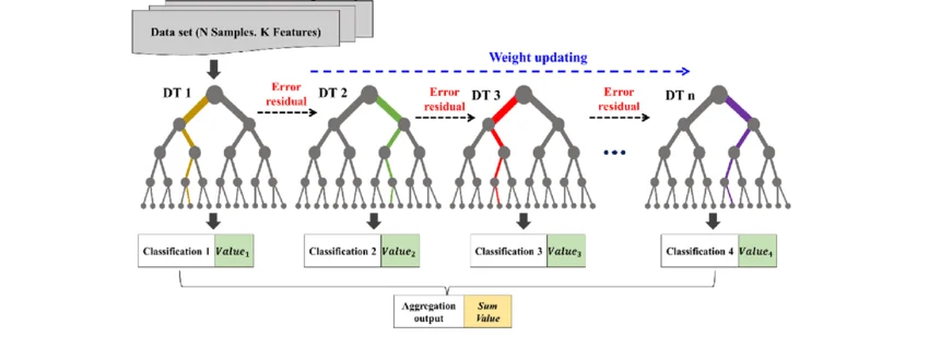
Step 1: Start with a Simple Baseline

The process starts by initializing an ensemble model $F_{0} (x)$ . This is typically a simple model predicts a value for all input data points.
- Regression: Usually the average of all target values
- Classification: Usually the log-odds (a way to represent probabilities)
This baseline is intentionally simple—we'll refine it through boosting

Iteration Loop: The algorithm then iterates $K$ times (where $K$ is the number of trees). Within each iteration:

Step 2: Calculate Pseudo-Residuals: (What Did We Get Wrong?)

For each training sample, compute: $Actual value - Current prediction$
These residuals represent how much our ensemble undershot or overshot
Example: If we predicted 100 but actual was 120, residual = +20
Example: If we predicted 80 but actual was 60, residual = -20

Step 3: Train a Tree to Predict Residuals

Build a decision tree that tries to predict these residuals
The tree learns patterns in what we're getting wrong
Key insight: The tree doesn't predict the original target—it predicts the errors!
Use a shallow tree (depth 3-6) to avoid overfitting

Step 4: Add This Tree to the Ensemble (With Caution)

Add the new tree's predictions to our ensemble
But multiply by a small learning rate (like 0.1) to be conservative
Why small steps?: Taking big jumps might overshoot and make things worse
Analogy: When adjusting a thermostat, you don't crank it to the max—you make small adjustments

The update looks like:
New prediction = Old prediction + (learning rate × tree prediction)

Step 5: Repeat with New Residuals

Calculate residuals based on the updated ensemble
Train another tree on these new residuals
Add it to the ensemble (again, multiplied by learning rate)
Continue for many iterations (typically 100-1000 trees)

Step 6: Final Prediction—Sum of All Corrections

Start with the baseline prediction
Add each tree's contribution (scaled by learning rate)
The final prediction is: Baseline + Tree₁ + Tree₂ + Tree₃ + ... + TreeN
Each tree contributed a small correction, and together they form an accurate prediction

》》》👉 Step by Step — Mathematical Derivation of GBM

Concrete Example—Predicting Age from Photos:

Round	Current Prediction	Actual Age	Residual	New Tree Learns	Updated Prediction
0	30 (baseline avg)	45	+15	"wrinkles" → +12	30 + 0.1×12 = 31.2
1	31.2	45	+13.8	"gray hair" → +10	31.2 + 0.1×10 = 32.2
2	32.2	45	+12.8	"posture" → +8	32.2 + 0.1×8 = 33.0
...	...	45	...	...	...
50	44.5	45	+0.5	(small corrections)	44.8

Each tree adds a small correction based on patterns in remaining errors. Over many rounds, we converge to accurate predictions.

Why This Works:

Early trees: Learn major patterns (obvious correlations)
Middle trees: Refine predictions (subtle interactions)
Later trees: Handle edge cases (fine-tuning)
Learning rate: Prevents any single tree from dominating
Shallow trees: Keep each correction simple and interpretable

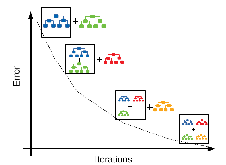
Gradient Boosting Characteristics

Strengths:

Highly flexible: Works with any differentiable loss function (squared error, log loss, custom losses)
Excellent performance: State-of-the-art on structured data for many years
Natural regularization: Learning rate prevents overfitting through small steps
Works for both: Classification and regression without significant changes
Handles various data types: Numerical, categorical, mixed features
Feature importance: Can extract which features matter most

Weaknesses:

More complex: More hyperparameters than AdaBoost (learning rate, tree depth, iterations)
Sequential bottleneck: Must train trees one at a time—can't parallelize across iterations
Hyperparameter sensitive: Performance varies significantly with different settings
Can overfit: Especially with too many iterations or trees that are too deep
Slower training: Sequential nature means training takes longer than bagging methods

Questions and Answers

The name "Gradient Boosting" comes from a precise connection to gradient descent. The insight is that fitting trees to residuals is literally performing gradient descent—not on the model's parameters, but on its predictions.

Recap of ordinary gradient descent.
When we minimize a loss $L (θ)$ over parameters $θ$ , we repeatedly step in the direction of the negative gradient:

θ \leftarrow θ - η \frac{\partial L}{\partial θ}

Each step nudges the parameters so that the loss decreases.

Gradient descent in "function space".
In boosting, we do not have a fixed set of parameters to tune. Instead, the thing we are optimizing is the prediction itself. Treat the $n$ predictions $F (x_{1}), \dots, F (x_{n})$ as the variables we can move freely, and consider the squared-error loss:

L = \frac{1}{2} \sum_{i = 1}^{n} (y_{i} - F (x_{i}))^{2}

Take the derivative of the loss with respect to a single prediction $F (x_{i})$ :

\frac{\partial L}{\partial F (x_{i})} = - (y_{i} - F (x_{i}))

The negative gradient is therefore:

- \frac{\partial L}{\partial F (x_{i})} = y_{i} - F (x_{i}) = {residual}_{i}

Residual = Negative Gradient

For squared-error loss, the residual $y_{i} - F (x_{i})$ is exactly the negative gradient of the loss with respect to the current prediction. So when a tree fits the residuals, it is estimating the direction of steepest descent in prediction space.

The parallel side by side:

Concept	Gradient Descent (parameters)	Gradient Boosting (functions)
What we optimize	Parameters $θ$	The model function $F (x)$
Quantity we move	$θ$	Predictions $F (x_{i})$
Direction of movement	$- \partial L / \partial θ$	$- \partial L / \partial F (x_{i})$ = residual
Step estimator	Compute gradient directly	Fit a weak learner to the gradient
Step size	Learning rate $η$	Learning rate $ν$ (shrinkage)
Update rule	$θ \leftarrow θ - η \nabla L$	$F \leftarrow F + ν h$

So each new tree $h$ is a step in the direction that most rapidly reduces the loss, and the learning rate controls how large that step is—exactly like gradient descent.

2. What is difference between AdaBoost and Gradient Boosting?

	AdaBoost	Gradient Boosting Machine (GBM)
Definition	Adaptive Boosting (AdaBoost) is an ensemble method that combines multiple "weak learners" (typically decision stumps/trees) sequentially, focusing on reweighting misclassified samples.	GBM is a general boosting framework that combines weak models (typically decision trees) by minimizing the loss function through gradient descent iterations.
The Core Difference	At each step, AdaBoost identifies the specific data points that were misclassified by the previous model and increases their weights. The next model is then forced to focus more heavily on getting those specific "hard-to-predict" points right.	GBM does not change the weights of the data points. Instead, it calculates the residuals (the difference between the actual value and the predicted value) of the previous model. The next model is then trained specifically to predict those errors/residuals, using a loss function (like Mean Squared Error) and gradient descent to minimize them.
Weak Learners Used	Typically uses very simple models, usually Decision Stumps (a decision tree with only one split/one level deep).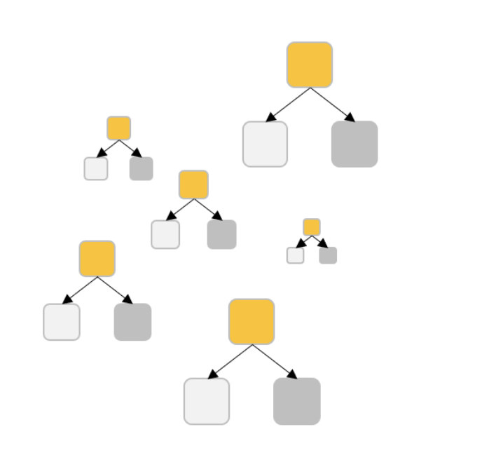	Uses slightly more complex models. While it also typically uses decision trees, they are usually grown deeper (e.g., 8 to 32 terminal nodes). Furthermore, GBM is flexible and can theoretically use linear models or other algorithms as base learners.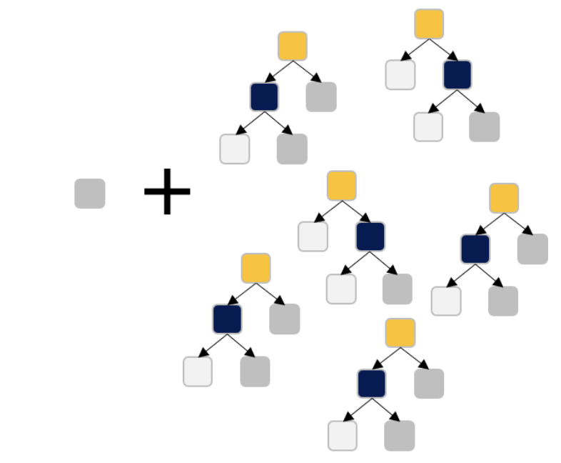
Weight Adjustment	In AdaBoost, weights are adjusted for the samples based on their classification error. Higher weights are assigned to misclassified samples so that the next weak learner focuses more on them.	GBM optimizes predictions by iteratively minimizing the gradient of a differentiable loss function. No direct sample weights adjustment.
Loss Function	Minimizes the exponential loss function: $$Loss = \sum e^{-\alpha_t y_i h_t(x_i)}$$ The focus is more on minimizing classification errors.	Can be customized for the task (e.g., squared error for regression, log-loss for classification). Optimizes via gradient descent.
Training Objective	Prioritizes misclassified examples by increasing their importance to the next weak learner.	Reduces the residual error of the model using gradient descent on the error at each step.
Interpretability	Slightly easier to interpret since it focuses on sample reweighting and decision stumps.	Harder to interpret due to the use of arbitrary loss functions and deeper decision trees.
Speed	Faster as it often uses shallow decision stumps.	Slower training compared to AdaBoost due to the iterative nature and use of deeper trees.
Handling of Outliers	Sensitive to outliers; assigns higher weight to misclassified samples, which includes outliers, potentially distorting the model.	Less sensitive to outliers; trees in GBM are constructed to minimize error for the entire dataset.
Customization	Limited customization options; primarily focuses on classification and sample weighting.	Highly customizable; supports various loss functions (e.g., regression, classification, ranking) and hyperparameter tuning.
Hyperparameters	Fewer hyperparameters (e.g., number of weak learners, learning rate).	Many hyperparameters (e.g., learning rate, tree depth, number of iterations) to tune for optimal performance.
Overfitting Control	Less prone to overfitting with simple decision stumps but becomes overfitting-prone with strong learners.	More prone to overfitting, especially with deeper trees. Regularization techniques (learning rate, subsampling) can mitigate this.
Dataset Size	Works well with small to medium-sized datasets.	Can handle large datasets effectively but might require tuning for optimal performance.
Applications	Best for classification tasks, especially binary classification.	Flexible: can be used for regression, classification, and even ranking tasks.
Algorithm Complexity	Conceptually simpler due to focus on reweighting and typically using simple learners.	More complex due to support for advanced optimization techniques and loss functions.
Implementation Complexity	Easier to implement due to limited configuration options.	More sophisticated and requires tuning to achieve optimal results.
Robustness to Noise	Less robust: sensitive to noisy data and outliers, as higher weights can be assigned to noisy samples.	More robust: less focus on individual misclassifications, reducing the effect of noisy data.

Gradient Boosting

Core Concept—Learning from Residuals

Background—The Problem Setup

How Gradient Boosting Works?

Gradient Boosting Characteristics

Questions and Answers

1. How Is This Related to Gradient Descent?

2. What is difference between AdaBoost and Gradient Boosting?