Decision Tree Classifier
A Decision Tree is a supervised machine learning algorithm that builds a flowchart-like tree structure to make predictions by recursively partitioning data based on the most informative feature at each step.
Decision trees create a model that predicts the label by evaluating a tree of if-then-else true/false feature questions, and estimating the minimum number of questions needed to assess the probability of making a correct decision.
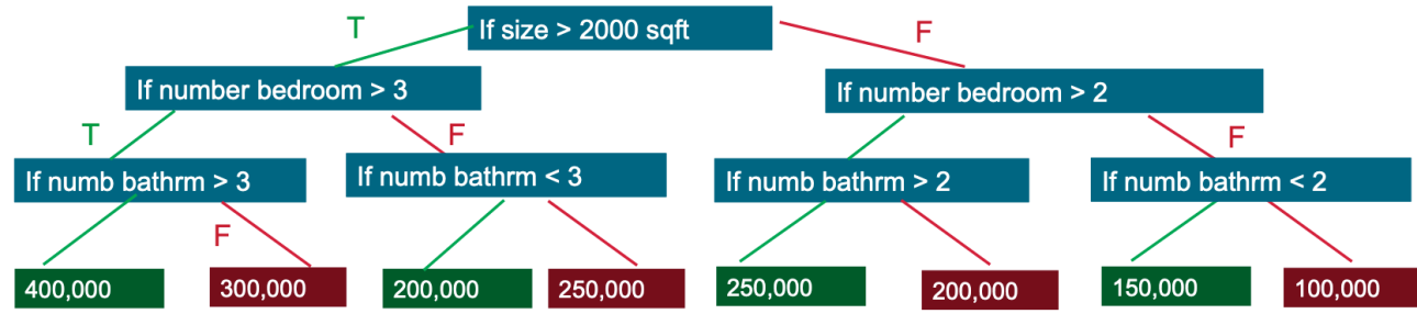
Decision trees can be used for classification to predict a category, or regression to predict a continuous numeric value. In the simple example below, a decision tree is used to estimate a house price (the label) based on the size and number of bedrooms (the features).
I. Components
| Component | Role |
|---|---|
| Root Node | Topmost node; represents the full dataset; holds the single best split |
| Internal (Decision) Node | Tests one feature (e.g., Age > 30?); routes samples left or right |
| Leaf (Terminal) Node | No further split; holds the predicted class label (majority class) |
| Branch / Edge | The outcome of a test (True / False, or a threshold range) |
II. Algorithm Steps
The algorithm is greedy and recursive: it makes the locally best split at every node without backtracking.
Step 1 – Start at the root with the full dataset.
Step 2 – For every feature, evaluate every possible split threshold and compute the impurity reduction (Information Gain):
Step 3 – Choose the feature + threshold that gives the highest Information Gain.
Step 4 – Split the data and create two child nodes (CART) or multiple children (ID3 / C4.5).
Step 5 – Recurse on each child node until a stopping criterion is met:
- Node is pure (all same class)
max_depthreachedmin_samples_split/min_samples_leafnot satisfiedmin_impurity_decreasethreshold not met
Step 6 – Assign the majority class of remaining samples to each leaf.
★ Algorithms used
| Algorithm | Split Type | Criterion | Pruning | Data Types | Used for | Outliers |
|---|---|---|---|---|---|---|
| CART (✅ Default) |
Binary only | Gini or MSE | Cost-Complexity | Numerical + Categorical | Classification, Regression | Very Robust |
| ID3 | Multi-way | Information Gain (Entropy) | Post-Pruning | Categorical only | Classification | Sensitive |
| C4.5 | Multi-way | Gain Ratio | Post-Pruning | Both | Classification, Regression | Sensitive |
| CHAID | Multi-way | Chi-Square / F-test | Pre-Pruning (Early Stop) | Both | Sensitive |
III. Split Criteria (Metrics)
Set via the criterion= parameter in DecisionTreeClassifier.
i. Gini Impurity — criterion="gini" (default)
- Range: 0 (pure) → 0.5 (binary, perfectly mixed)
- Intuition: Probability of incorrectly labelling a randomly picked sample using the node's class distribution.
- Speed: ⚡ Fastest — no logarithm required.
Use when: General-purpose classification; default choice; speed matters.
ii. Entropy — criterion="entropy"
- Range: 0 (pure) → 1 (binary, perfectly mixed) →
(C-class max) - Intuition: Average information needed to identify the class of a sample — measures disorder.
- Speed: ~10–20% slower than Gini due to log calculation.
Use when: You want information-theoretic splits; studying feature selection; replicating ID3/C4.5 behaviour.
📌 In practice: Gini and Entropy almost always produce near-identical trees and accuracy. Start with Gini; switch to Entropy only if cross-validation shows a meaningful difference.
iii. Log Loss — criterion="log_loss" (sklearn ≥ 1.1)
- Intuition: Penalises confident wrong predictions heavily; directly optimises probability calibration rather than classification boundaries.
- Speed: Slowest of the three.
Use when: You need well-calibrated probabilities for downstream use — risk scoring, medical diagnosis, cost-sensitive decisions where predict_proba output matters more than raw accuracy.
IV. Binary vs. Multi-way Splits
i. Binary Split (CART — sklearn default)
Every node asks exactly one yes/no question. Categorical features are tested as feature ∈ {subset} vs feature ∉ {subset}.
- Produces a deeper but narrower tree.
- Lower overfitting risk — small categories get grouped together rather than isolated branches.
Outlook == Overcast?
   ├── Yes → [Pure: Play=Yes]  ✓ Stop
   └── No  → [Mixed: Sunny + Rainy] → split further
Sklearn: ✅ Supported
ii. Multi-way Split (ID3 / C4.5 / CHAID)
Creates one branch per unique value of the chosen feature simultaneously.
- Produces a wider but shallower tree.
- Higher overfitting risk — high-cardinality features produce many tiny, pure branches that don't generalize.
Outlook?
   ├── Sunny    → [Mixed] → split further
   ├── Overcast → [Pure: Play=Yes] ✓ Stop
   └── Rainy    → [Mixed] → split further
Sklearn: ❌ Not supported
V. Pros and Cons
| ✅ Pros | ⚠️ Cons |
|---|---|
| Highly interpretable — visualise and explain to non-experts | Unstable — small data changes can produce a completely different tree |
| No feature scaling required | Prone to overfitting — unbounded trees memorise noise |
| Handles numerical and categorical data | Greedy — local optimal splits do not guarantee the globally best tree |
| Fast to train and predict | Biased toward high-cardinality features (especially with entropy/ID3) |
| Captures non-linear relationships naturally | Axis-aligned decision boundaries — struggles with diagonal patterns |
| Natural multi-class support | Large trees become hard to interpret |
| Provides feature importances | High variance — single DTs are weak learners, hence used in ensembles (RF, XGBoost) |
VI. Code Examples
- Train, Evaluate & Visualise:
- Bias–Variance Plot: Sweeping max_depth:
- Post-Pruning: ccp_alpha Path:
- GridSearchCV Hyperparameter Tuning:
- Feature Importance Plot:
Key attributes available after fitting:
clf.tree_.max_depth        # actual depth reached
clf.get_depth()            # same via public API
clf.get_n_leaves()         # number of leaf nodes
clf.feature_importances_   # Gini-based importance per feature
clf.classes_               # class labels in order
VII. Overfitting, Bias–Variance Trade-Off & pruning
VIII. Questions and Answers
1. How to pick the values for class_weight?
Option A: The "Balanced" Auto-Pilot (Recommended)
Most libraries (like Scikit-Learn) have a built-in setting called class_weight='balanced'.
The Formula:
It automatically calculates weights inversely proportional to class frequencies:
- Example: If you have 100 samples (90 "Safe", 10 "Risk"):
- Weight for Safe:
- Weight for Risk:
- Weight for Safe:
- Result: The model treats each "Risk" instance as being
more important than a "Safe" instance.
Option B: Manual "Cost-Based" Weighting
Sometimes "Balanced" isn't enough. In finance, the cost of a False Negative (missing a default) is much higher than a False Positive (denying a good loan).
You can pass a dictionary: class_weight={0: 1, 1: 20}.
- Pick this when you have a specific Business Cost associated with an error. If a missed "Class 1" event costs the firm
and a false alarm costs , a ratio is mathematically sound.
2. How manually setting class_weight changes the Math (Gini/Entropy)?
When you add weights, the "Purity" calculation changes.
Instead of:
It becomes: