Geometric Distance Metrics

1. Euclidean Distance (L2 Norm)

The Euclidean distance is the most widely used distance metric in machine learning, especially in K-means clustering. It calculates the straight-line distance between two data points in vector space.

👉 Euclidean Distance is like like measuring with a ruler

Formula for 'n' dimensions

For two points $P = (x_{1}, x_{2}, . . ., x_{n})$ and $Q = (y_{1}, y_{2}, . . ., y_{n})$ , the Euclidean distance $d (P, Q)$ is defined as:

d (P, Q) = \sqrt{\sum_{i = 1}^{n} (x_{i} - y_{i})^{2}}

Component Breakdown:

$x_{i}$ and $y_{i}$ : Coordinates of the two points $P$ and $Q$ in $n$ -dimensional space
$\sum_{i = 1}^{n}$ : Summation over all $n$ dimensions (features)
$(x_{i} - y_{i})^{2}$ : Squared difference between corresponding coordinates (ensures positive values)
$\sqrt{\cdot}$ : Square root gives actual distance (otherwise it's squared Euclidean distance)

Visual Representation in 2D:

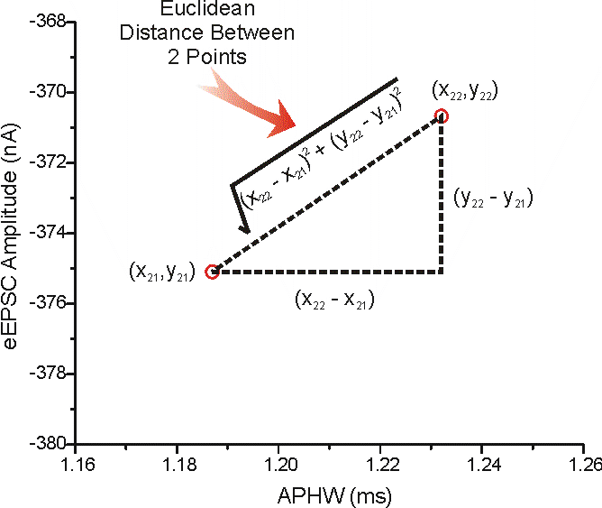
Example in 2D:

$P = (3, 4), Q = (0, 0)$
$d (P, Q) = \sqrt{(3 - 0)^{2} + (4 - 0)^{2}} = \sqrt{9 + 16} = \sqrt{25} = 5$

👉 In K-Means: Point $Q$ represents the cluster centroid, and we minimize the sum of squared Euclidean distances

When to Use:

Features are continuous and on similar scales
Data is relatively normally distributed
All features have equal importance
You need intuitive, geometric distance

Advantages:

✅ Intuitive and geometrically meaningful
✅ Directly optimized in K-Means
✅ Works well with compact, spherical clusters

Disadvantages:

❌ Sensitive to scale: Features with larger ranges dominate the distance
❌ Curse of dimensionality: Becomes less meaningful in very high dimensions
❌ Sensitive to outliers: Squared differences amplify large deviations
❌ Assumes feature independence: Doesn't account for correlations

Practical Tips:

Always standardize/normalize features before using Euclidean distance
Consider using Mahalanobis distance if features are correlated
Use Manhattan distance if you want to reduce outlier sensitivity

❗ What’s wrong with using Euclidean Distance for Multivariate data?

Euclidean distance does not account for correlations among features

1. Euclidean Distance Ignores Correlation:

Euclidean distance only measures the straight-line distance between two points, without considering relationships between dimensions (features). However, in real-world datasets, features are often correlated or dependent on one another (e.g., height and weight, or income and spending habits).

2. Misleading Interpretation in Correlated Data

When features are positively or negatively correlated, data points form an elliptical distribution rather than a spherical one. In such cases, Euclidean distance assumes the points are distributed equally in all directions, leading to misleading distance measurements.

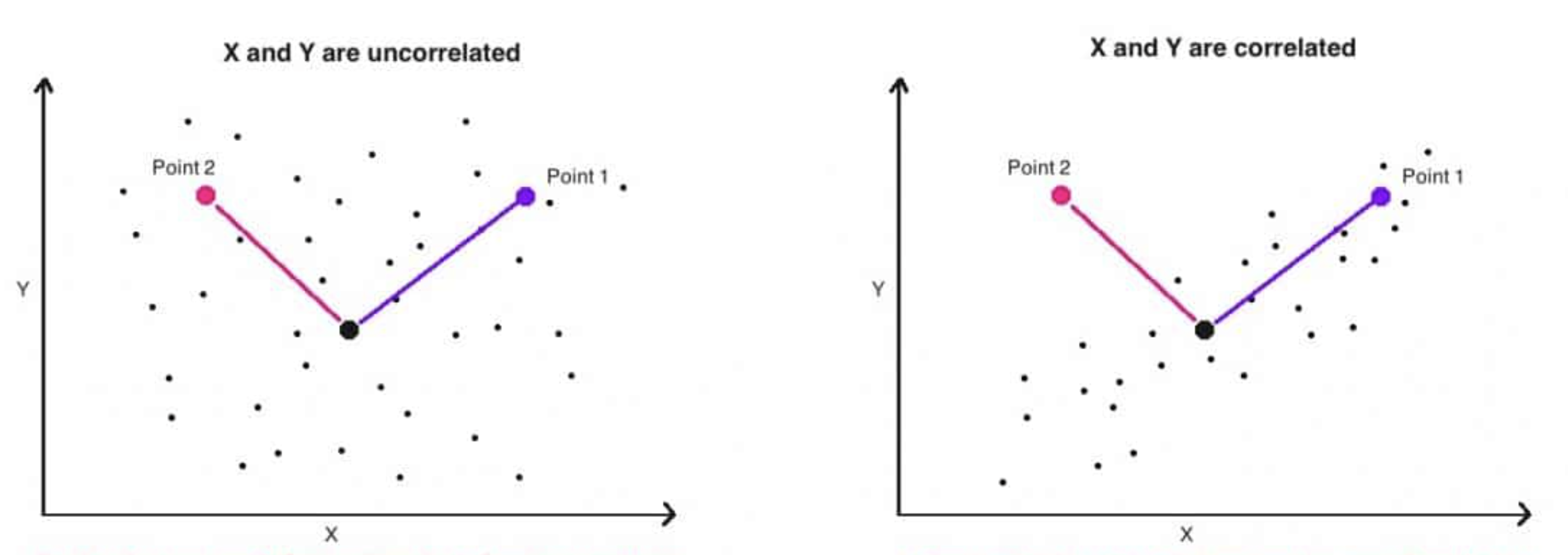
Illustration of Correlated Data

Uncorrelated Data (Left Plot)
When Point 1 and Point 2 are uncorrelated (points are distributed uniformly in all directions): The Euclidean distance is effective because it directly measures the proximity of a point to the cluster's centroid.
Correlated Data (Right Plot)
When Point 1 and Point 2 are correlated (e.g., points tend to form an elliptic cluster):
- Both Point 1 (inside the cluster) and Point 2 (outlier) can have identical Euclidean distances to the centroid.
  - Point 1 (purple) aligns with the direction of the cluster (along the ellipse's major axis).
  - Point 2 (pink) deviates significantly from the cluster because it goes against the natural direction of the data variance.
Despite its deviation, Euclidean distance cannot capture this, making Point 2 look just as close to the cluster as Point 1.

Why Does This Happen?

Euclidean distance ignores the distribution of other points in the dataset. It only considers the distance between two individual points and doesn't account for how the rest of the points vary. Essentially:

It assumes the data is spherically symmetric (same variance in all directions).
It ignores the spread and correlation structure of the data, which are critical in identifying clusters or determining whether a point is an outlier.

The Solution: Use Mahalanobis Distance

The Mahalanobis Distance is a more robust alternative for measuring the distance of a point from a cluster when dealing with correlated data. It considers the distribution of the entire dataset.

2. Manhattan Distance (L1 Norm)

The Manhattan Distance (also called Taxicab Distance, City Block Distance, or L1 norm) measures the distance between two points by summing the absolute differences of their coordinates. It mimics navigating a grid-like city street layout where you can only move horizontally or vertically.

Formula for 'n' dimension

For two points $P = (x_{1}, x_{2}, \dots, x_{n})$ and $Q = (y_{1}, y_{2}, \dots, y_{n})$ in an $n$ -dimensional space:

d (P, Q) = \sum_{i = 1}^{n} | x_{i} - y_{i} |

Component Breakdown:

$| x_{i} - y_{i} |$ : Absolute difference (no squaring, unlike Euclidean)
$\sum_{i = 1}^{n}$ : Sum over all dimensions
No square root needed (simpler computation)

Example in 2D:

$P = (3, 4), Q = (1, 1)$
$d (P, Q) = | 3 - 1 | + | 4 - 1 | = 2 + 3 = 5$

Visual Comparison (2D example):

Euclidean: $d = \sqrt{2^{2} + 3^{2}} = \sqrt{13} \approx 3.61$ (diagonal line)
Manhattan: $d = 2 + 3 = 5$ (grid path)

When to Use:

Features are on different scales (more robust than Euclidean)
Data has outliers (less sensitive than Euclidean)
Grid-like or discrete data structures
You want to reduce the impact of large differences in any single dimension

Advantages:

✅ Less sensitive to outliers than Euclidean
✅ Faster to compute (no squaring or square root)
✅ More robust when features have different scales
✅ Natural for grid-based problems

Disadvantages:

❌ Less intuitive than Euclidean distance
❌ Not differentiable at zero (problematic for some optimization algorithms)
❌ May overestimate distances in high dimensions

Applications:

Machine Learning: KNN, K-Medians clustering, LASSO regression (L1 regularization)
Robotics/Pathfinding: A* algorithm on grid maps
Image Processing: Comparing pixel intensities, image histograms
Recommendation Systems: Similarity with categorical or ordinal features

3. Chebyshev Distance

Chebyshev distance (or $L_{\infty}$ metric) is a distance measure defined as the maximum absolute difference between corresponding coordinates of two vectors.
It assumes the moment can occur in any direction including diagnols.

This distance is especially useful in grid-based systems like chessboards or pathfinding in games where diagonal movement is allowed.

Formula

For points $P = (x_{1} , x_{2} , . . ., x_{n} )$ and $Q = (y_{1}, y_{2}, . . ., y_{n})$

D_{C h e b y s h e v} (P, Q) = \sum_{i = 1}^{n} m a x (| x_{i} - y_{i} |)

Component Breakdown:

$| x_{i} - y_{i} |$ : Absolute difference (no squaring, unlike Euclidean)
$\sum_{i = 1}^{n}$ : Sum over all dimensions
No square root needed (simpler computation)
Maximum of all Absolute difference

Visual Example in 2D

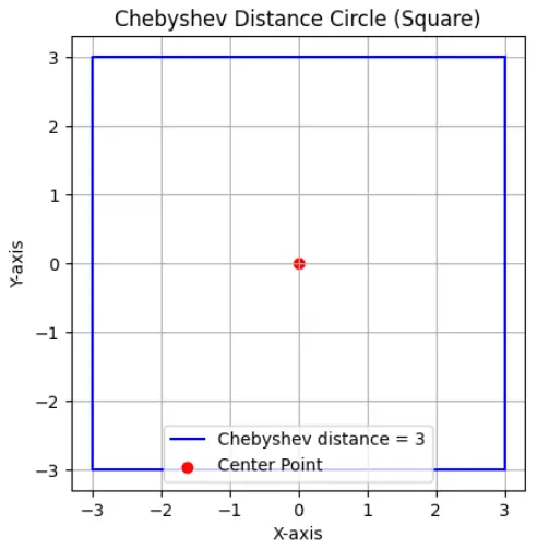
Example in 2D
Consider 2 points: $X = (0, 0)$ , $Y = (- 2, - 3)$

\begin{aligned} d_{C h e b y s h e v} (X, Y) & = max (| 0 - (- 2) |, | 0 - (- 3) |) \\ = max (2, 3) = 3 \end{aligned}

The plot shows a square centered at (0,0) representing all points exactly 3 units away by Chebyshev distance.

Advantages:

✅ Very fast to compute: Only need to find maximum, no summation or square roots
✅ Intuitive for grid-based problems: Natural for chessboard and warehouse movements
✅ Focuses on bottleneck: Identifies the limiting dimension
✅ Memory efficient: Only need to track one value (the max)

Disadvantages:

❌ Ignores small differences: Only the largest dimension matters, losing other information
❌ Poor for clustering: Not suitable for most ML algorithms like K-Means
❌ Less intuitive in continuous space: Works better for discrete grids
❌ Sensitive to single outlier dimension: One extreme coordinate can dominate
❌ Limited ML applications: Rarely used in standard clustering/classification

Applications:

Game AI & Robotics:
- Chess king movement, pathfinding with diagonal moves
- Grid-based robot navigation where diagonal movement has equal cost
Logistics & Operations:
- Warehouse optimization (slowest worker determines completion time)
- Scheduling problems (bottleneck identification)
Image Processing:
- Pixel neighborhood analysis (8-connectivity)
- Maximum color channel difference detection
Quality Control:
- Manufacturing tolerance checks (worst-case dimension)
- Identifying the most deviant measurement

4. Minkowski Distance (Generalized Lp Norm)

Minkowski distance is a generalized metric used to calculate the distance between two points in
$n$ -dimensional space, unifying measures like Euclidean and Manhattan distances. It is defined by a parameter $p$ (order), where higher $p$ values change how coordinate differences are weighted. It is widely applied in machine learning for clustering (k-means) and classification (
K-NN)

Formula

For two points $P = (x_{1}, x_{2}, \dots, x_{n})$ and $Q = (y_{1}, y_{2}, \dots, y_{n})$ :

d (P, Q) = {(\sum_{i = 1}^{n} | x_{i} - y_{i} |^{p})}^{1 / p}

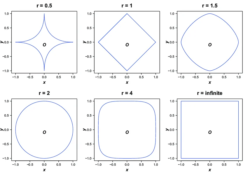
Special Cases:

$p = 1$ : Manhattan Distance (L1 norm)
$p = 2$ : Euclidean Distance (L2 norm)
$p = \infty$ : Chebyshev Distance (maximum absolute difference): $max_{i} | x_{i} - y_{i} |$

Example ( $P = (3, 4)$ , $Q = (0, 0)$ ):

$p = 1$ : $d = | 3 | + | 4 | = 7$ (Manhattan)
$p = 2$ : $d = \sqrt{3^{2} + 4^{2}} = 5$ (Euclidean)
$p = 3$ : $d = (3^{3} + 4^{3})^{1 / 3} = (27 + 64)^{1 / 3} = 91^{1 / 3} \approx 4.50$
$p = \infty$ : $d = max (3, 4) = 4$ (Chebyshev)

When to Use:

Experiment with different $p$ values to find what works best for your data
Higher $p$ values give more weight to larger differences
Lower $p$ values are more robust to outliers

Visualization:

➢ Euclidean vs Manhattan vs Chebyshev

1. Side-by-Side View

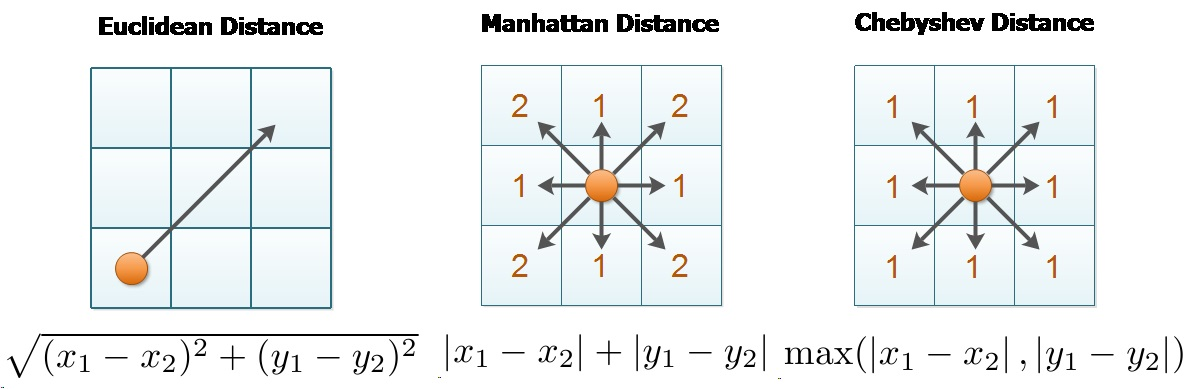
2. Overlay View: Assuming (0,0) as a one of the point

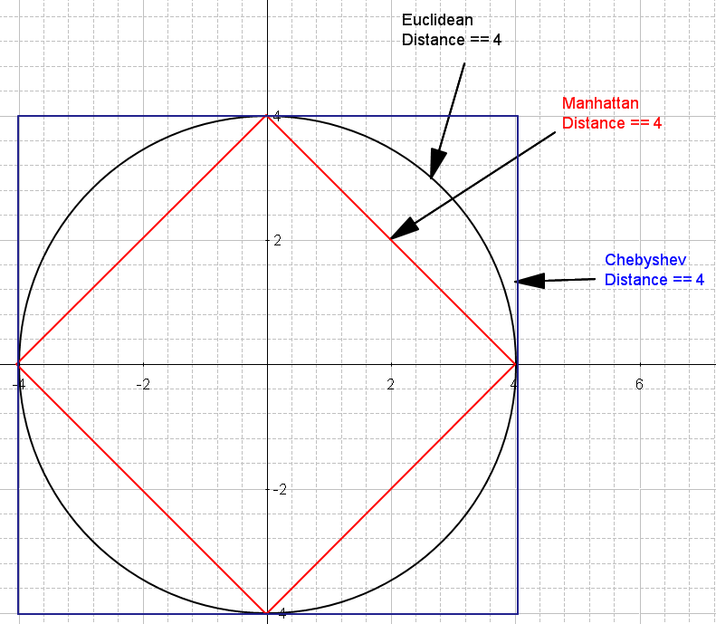
Euclidean: A circle (all points equidistant)
Manhattan: A diamond (rotated square)
Chebyshev: A square aligned with axes

Comparison (for $P = (3, 4)$ , $Q = (1, 1)$ ):

Euclidean: $d = \sqrt{2^{2} + 3^{2}} = \sqrt{13} \approx 3.61$
Manhattan: $d = | 2 | + | 3 | = 5$
Chebyshev: $d = max (2, 3) = 3$