Activation Functions in Neural Networks

Activation functions are mathematical operations applied to neurons in a neural network that introduce non-linearity, enabling the network to learn complex patterns and relationships in data. Without activation functions, neural networks would be limited to learning only linear transformations, regardless of depth.

Formal Definition

An activation function is a mathematical function $f : R \to R$ (or $f : R \to (a, b)$ ) that transforms the weighted sum of inputs to a neuron, introducing non-linearity into the network and determining the neuron's output signal.

Given weighted sum $z = \sum_{i = 1}^{n} w_{i} x_{i} + b$ , the neuron's output is: $a = f (z)$

I. Fundamental Concepts

1. What are the main purposes of Activation Functions?

Activation functions are mathematical transformations applied at each neuron that determine:

Whether a neuron should activate (fire a signal)
The strength of the activation (output magnitude)
What information propagates to subsequent layers

Think of activation functions as decision gates that control information flow through the network.

2. The Neuron's Computation Pipeline

Every neuron performs a two-step process:

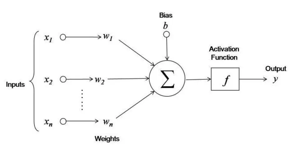
Step 1: Linear Aggregation (Pre-activation)

z = w_{1} x_{1} + w_{2} x_{2} + \dots + w_{n} x_{n} + b = w^{T} x + b

Where:

$x = [x_{1}, x_{2}, . . ., x_{n}]$ = Input vector
$w = [w_{1}, w_{2}, . . ., w_{n}]$ = Weight vector (learnable parameters)
$b$ = Bias term (learnable parameter)
$z$ = Pre-activation value (weighted sum)

Step 2: Non-Linear Transformation (Activation)

a = f (z)

Where:

$f$ = Activation function
$a$ = Activation value (neuron's output)

3. Information Flow Through Layers

In Hidden Layers:

Neuron output $a^{[l]}$ becomes input $x^{[l + 1]}$ for the next layer
Notation: $a_{j}^{[l]}$ = activation of neuron $j$ in layer $l$

In Output Layer:

Final activation $a^{[L]}$ = network's prediction
Choice of activation depends on the task (classification, regression, etc.)

II. Mathematical Foundation

1. Why Do We Need Activation Functions?

The Linearity Trap:

Without activation functions, a neural network—regardless of its depth—collapses into a single linear transformation.

Mathematical Proof:
Consider a 3-layer network with only linear operations:

\begin{aligned} Layer 1: & h_{1} & = W_{1} x + b_{1} \\ Layer 2: & h_{2} & = W_{2} h_{1} + b_{2} = W_{2} (W_{1} x + b_{1}) + b_{2} \\ Layer 3: & y & = W_{3} h_{2} + b_{3} = W_{3} [W_{2} (W_{1} x + b_{1}) + b_{2}] + b_{3} \end{aligned}

Expanding:

y = W_{3} W_{2} W_{1} x + W_{3} W_{2} b_{1} + W_{3} b_{2} + b_{3}

This simplifies to:

y = W^{'} x + b^{'}

Where $W^{'} = W_{3} W_{2} W_{1}$ and $b^{'} = W_{3} W_{2} b_{1} + W_{3} b_{2} + b_{3}$

Conclusion: A deep linear network = a single linear layer (no benefit from depth!)

2. Non-Linearity: The Game Changer

Activation functions introduce non-linearity through:

Sigmoid: Creates S-shaped curves (smooth squashing)
ReLU: Creates piecewise linear boundaries (sharp corners)
Tanh: Creates symmetric S-curves (zero-centered)

Impact on Decision Boundaries:

Linear networks: Can only separate classes with straight hyperplanes
Non-linear networks: Can form arbitrarily complex decision boundaries (curves, circles, spirals)

3. The Role of Derivatives in Learning (Backpropagation)

Neural networks learn through gradient descent, which requires computing gradients of the loss function with respect to all parameters.

The Chain Rule in Action:
To update weight $w_{i j}^{[l]}$ connecting neuron $i$ in layer $l - 1$ to neuron $j$ in layer $l$ :

\frac{\partial L}{\partial w_{i j}^{[l]}} = \frac{\partial L}{\partial a_{j}^{[l]}} \times \frac{\partial a_{j}^{[l]}}{\partial z_{j}^{[l]}} \times \frac{\partial z_{j}^{[l]}}{\partial w_{i j}^{[l]}}

Where:

$\frac{\partial L}{\partial a_{j}^{[l]}}$ = Error signal from subsequent layers
$\frac{\partial a_{j}^{[l]}}{\partial z_{j}^{[l]}} = f^{'} (z_{j}^{[l]})$ = Derivative of activation function (critical!)
$\frac{\partial z_{j}^{[l]}}{\partial w_{i j}^{[l]}} = a_{i}^{[l - 1]}$ = Input from previous layer

Key Insight: The activation function's derivative $f^{'} (z)$ directly controls gradient flow!

4. Gradient Pathologies

Vanishing Gradients:

Problem: When $| f^{'} (z) | ≪ 1$ (close to 0), gradients shrink exponentially through layers
Effect: Early layers learn extremely slowly or not at all
Culprits: Sigmoid, Tanh (derivatives peak at 0.25 and 1, respectively)
Formula: If each layer has gradient 0.25, after 10 layers: $(0.25)^{10} \approx 10^{- 6}$

Exploding Gradients:

Problem: When $| f^{'} (z) | ≫ 1$ , gradients grow exponentially
Effect: Weights oscillate wildly, training becomes unstable
Solution: Gradient clipping, careful initialization, batch normalization

Dead Neurons (Dying ReLU):

Problem: When $z < 0$ always, ReLU outputs 0, and $f^{'} (z) = 0$
Effect: Neuron stops learning permanently (gradient is always 0)
Cause: Poor initialization, high learning rates
Solution: Leaky ReLU, proper initialization (He initialization)

III. Activation Functions Catalog

1. Linear Activation

Function	Derivative
$$\large f(z) = mz$$ where $m$ is a constant (usually 1)	$$f'(z) = m$$

Mathematical Properties:

Range: $(- \infty, \infty)$
Derivative: Constant (independent of input)
Continuity: Continuous and differentiable everywhere

Advantages:

✅ Simple and fast to compute
✅ Provides continuous range of activations
✅ Suitable for regression output layers

Disadvantages:

❌ No non-linearity (network collapses to single layer)
❌ Gradient doesn't depend on input (poor learning dynamics)
❌ Cannot learn complex patterns
❌ Stacking linear layers provides no benefit

Use Cases:

✅ Regression ("output layer") (predicting continuous, unbounded values)
❌ Hidden layers (defeats the purpose of deep networks)

Key Insight

Always remember why linear activations defeat the purpose of deep networks in hidden layers. The key is that composition of linear functions is still linear.

2. Sigmoid (Logistic Function)

Function	Derivative
$$\sigma(z)=\frac{1}{1+e^{-z}}$$	$$\sigma'(z)=\sigma(z) \cdot (1-\sigma(z))$$

Mathematical Properties:

Range: $(0, 1)$
Shape: S-curve (smooth squashing function)
Derivative: Maximum at $z = 0$ where $σ^{'} (0) = 0.25$
Saturation: Both extremes ( $z \to \pm \infty$ ) approach constant values

Advantages:

✅ Smooth and differentiable everywhere
✅ Output interpretable as probability
✅ Bounded output (prevents extreme values)
✅ Biologically inspired (similar to neuron firing rates)

Disadvantages:

❌ Vanishing gradient problem: For $| z | > 5$ , $σ^{'} (z) \approx 0$ (gradient vanishes)
❌ Not zero-centered: All outputs are positive, causing zig-zagging gradients
❌ Computationally expensive: Requires exponential calculation
❌ Output saturation: Small changes in input cause negligible output change at extremes

Gradient Analysis:

At $z = 0$ : $σ^{'} (0) = 0.25$ (maximum gradient)
At $z = \pm 3$ : $σ^{'} (z) \approx 0.045$ (only 18% of maximum)
At $z = \pm 5$ : $σ^{'} (z) \approx 0.0066$ (only 2.6% of maximum)

Use Cases:

✅ Binary classification output layer (probability between 0 and 1)
✅ Multi-label classification output (independent probabilities per label)
✅ Gate mechanisms in LSTMs and GRUs (controlling information flow)
❌ Hidden layers of deep networks (vanishing gradient issue)
❌ Multi-class single-label classification (use Softmax instead)
❌ Regression tasks with unbounded output (use linear activation)

Key Insight to remember

Why sigmoid causes vanishing gradients mathematically
The "not zero-centered" problem and its impact on learning
Why it's still perfect for binary classification outputs
The relationship between sigmoid and binary cross-entropy loss

3. Softmax (Multi-Class Output)

Formula	Derivative
For output vector $z = [z_{1}, z_{2}, . . ., z_{K}]$ : $$\text{Softmax}(z_i) = \frac{e^{z_i}}{\sum_{j=1}^{K} e^{z_j}}$$	$$\frac{\partial \text{Softmax}(z_i)}{\partial z_j} = \text{Softmax}(z_i)(\delta_{ij} - \text{Softmax}(z_j))$$ where $δ_{i j}$ is the Kronecker delta

Mathematical Properties:

Range: $(0, 1)$ for each class
Constraint: $\sum_{i = 1}^{K} Softmax (z_{i}) = 1$ (valid probability distribution)

Advantages:

✅ Converts logits to valid probability distribution
✅ Mutually exclusive classes (higher value for one class suppresses others)
✅ Differentiable and works well with cross-entropy loss
✅ Interpretable outputs (direct probabilities)

Disadvantages:

❌ Only for output layer: Never use in hidden layers (destroys inter-layer information)
❌ Sensitive to outliers: Large $z_{i}$ dominates exponentially
❌ Computationally expensive: Multiple exponential operations
❌ Numerical instability: Large values can cause overflow

Numerical Stabilization:
To prevent overflow, subtract the maximum value before computing:

Softmax (z_{i}) = \frac{e^{z_{i} - max (z)}}{\sum_{j = 1}^{K} e^{z_{j} - max (z)}}

Use Cases:

✅ Multi-class single-label classification (e.g., digit recognition: 0-9)
✅ Exclusive class prediction (choose exactly 1 from N classes)
✅ Attention mechanisms in transformers (probability distribution over tokens)
❌ Multi-label classification (use Sigmoid per class - labels not mutually exclusive)
❌ Hidden layers (destroys information and gradient flow)

Key Insight to remember

The difference between Softmax (mutually exclusive) and Sigmoid (independent)
Why Softmax is used with categorical cross-entropy loss
The numerical stabilization trick
When to use Softmax vs multiple Sigmoid outputs

4. Tanh (Hyperbolic Tangent)

Function	Derivative
$$\tanh(z) = \frac{e^z - e^{-z}}{e^z + e^{-z}} = \frac{2}{1 + e^{-2z}} - 1$$	$$\tanh'(z) = 1 - \tanh^2(z)$$

Mathematical Properties:

Range: $(- 1, 1)$
Shape: S-curve centered at zero
Derivative: Maximum at $z = 0$ where $\tanh^{'} (0) = 1$
Symmetry: Odd function: $\tanh (- z) = - \tanh (z)$

Advantages:

✅ Zero-centered: Helps with gradient flow (better than Sigmoid)
✅ Stronger gradients than Sigmoid (derivative peaks at 1 vs 0.25)
✅ Symmetric around origin (balanced positive/negative outputs)
✅ Better for optimization in shallow networks

Disadvantages:

❌ Still suffers from vanishing gradients at extreme values
❌ Computationally expensive: Exponential operations
❌ Saturates for $| z | > 3$

Use Cases:

✅ Hidden layers in shallow networks (better than Sigmoid)
✅ Recurrent Neural Networks (RNNs, LSTMs, GRUs): Standard for hidden states
✅ Zero-centered data requirements: When you need symmetric outputs
✅ Output layer for targets in [-1, 1]: e.g., scaled regression
❌ Very deep networks (>10 layers): Use ReLU instead (vanishing gradient issue)
❌ Binary classification output: Use Sigmoid (need [0,1] for probability)

Key Insights to remember

Why Tanh is better than Sigmoid for hidden layers (zero-centered, stronger gradients)
The relationship: $\tanh (z) = 2 σ (2 z) - 1$
Why it's preferred in RNNs over Sigmoid
When vanishing gradients still occur despite improvements over Sigmoid

5. ReLU (Rectified Linear Unit)

Function	Derivative
$$\text{ReLU}(z) = \max(0, z) = \begin{cases} z & \text{if } z > 0 \ 0 & \text{if } z \leq 0 \end{cases}$$	$$\text{ReLU}'(z) = \begin{cases} 1 & \text{if } z > 0 \ 0 & \text{if } z \leq 0 \end{cases}$$

Mathematical Properties:

Range: $[0, \infty)$
Shape: Piecewise linear (corner at origin)
Derivative: Binary (0 or 1)
Not differentiable at $z = 0$ (but we use subgradient in practice)

Advantages:

✅ Computationally efficient: Just $max (0, z)$ —no exponentials!
✅ No vanishing gradient for positive values ( $f^{'} (z) = 1$ )
✅ Sparse activation: Only ~50% of neurons activate (efficient, prevents co-adaptation)
✅ Biologically realistic: Similar to neuron firing patterns
✅ Faster convergence: In practice, networks train 6x faster than with Sigmoid/Tanh
✅ Scale-invariant: Output scales linearly with input for positive values

Disadvantages:

❌ "Dying ReLU" problem: Neurons can get stuck at 0 forever
❌ Not zero-centered: All outputs are non-negative
❌ Unbounded: Can lead to exploding activations (mitigated by batch normalization)
❌ Not differentiable at $z = 0$ (theoretical issue, ignored in practice)

The Dying ReLU Problem:

Cause: If a neuron's weights get updated such that $z < 0$ for ALL inputs:
- Gradient becomes 0
- Weights never update again
- Neuron is "dead"
Common scenarios:
- High learning rates
- Poor initialization
- Large negative bias
Symptoms: After training, 20-40% of neurons always output 0

Use Cases:

✅ Default choice for hidden layers in deep networks
✅ Convolutional Neural Networks (CNNs): Industry standard for vision
✅ Deep networks (10+ layers): Prevents vanishing gradients
✅ When you need speed: Fastest activation to compute
❌ Output layers: Use Sigmoid (binary), Softmax (multi-class), or Linear (regression)
❌ When dying ReLU is observed: Switch to Leaky ReLU or ELU

Initialization Recommendation:

Use He initialization with ReLU: $W \sim N (0, \sqrt{2 / n_{i n}})$
Prevents neurons from dying at initialization

Key Insights to remember

Why ReLU doesn't suffer from vanishing gradients (for positive values)
The dying ReLU problem and how to detect/prevent it
Why it's computationally efficient compared to Sigmoid/Tanh
The concept of sparse activation and why it's beneficial
Proper initialization strategies (He initialization)

6. Leaky ReLU

Function	Derivative
$$\text{LeakyReLU}(z) = \begin{cases} z & \text{if } z > 0 \ \alpha z & \text{if } z \leq 0 \end{cases}$$ where $α$ is a small constant (typically 0.01)	$$\text{LeakyReLU}'(z) = \begin{cases} 1 & \text{if } z > 0 \ \alpha & \text{if } z \leq 0 \end{cases}$$

Mathematical Properties:

Range: $(- \infty, \infty)$
Shape: Piecewise linear with small negative slope
Derivative: Never exactly zero
Parameter: $α$ typically set to 0.01

Advantages:

✅ Fixes dying ReLU: Small gradient for negatives keeps neurons alive
✅ Computationally efficient: Still very fast (no exponentials)
✅ All ReLU benefits: Plus allows negative values to contribute
✅ Better gradient flow: Never completely blocks gradients

Disadvantages:

❌ Inconsistent results: Sometimes outperforms ReLU, sometimes not
❌ Requires tuning $α$ : (though default 0.01 usually works)
❌ Slightly more expensive: Than pure ReLU (negligible)
❌ Not zero-centered: Still outputs non-negative for positive inputs

Use Cases:

✅ When ReLU causes dying neurons: First alternative to try
✅ Deep networks: Where gradient flow is critical
✅ GANs (Generative Adversarial Networks): Especially in discriminator
✅ High learning rates: Makes network more robust to large updates
✅ Regression with negative outputs: When output can be negative

Variants:

Parametric ReLU (PReLU):
- $α$ is learned during training
- Formula: $PReLU (z) = max (α z, z)$
- One $α$ per channel/neuron
Randomized Leaky ReLU (RReLU):
- $α$ is random during training, fixed during testing
- Formula: $α \sim U (l, u)$ where $l < u$ (e.g., $l = 1 / 8, u = 1 / 3$ )
- Acts as regularization

Key Insights to remember

How Leaky ReLU solves the dying ReLU problem
The trade-off: slight increase in computation for better gradient flow
When to use standard ReLU vs Leaky ReLU
The difference between Leaky ReLU, PReLU, and RReLU
Why it's popular in GANs

7. ELU (Exponential Linear Unit)

Function	Derivative
$$\text{ELU}(z) = \begin{cases} z & \text{if } z > 0 \ \alpha(e^z - 1) & \text{if } z \leq 0 \end{cases}$$ where $α > 0$ (typically 1.0)	$$\text{ELU}'(z) = \begin{cases} 1 & \text{if } z > 0 \ \alpha e^z = \text{ELU}(z) + \alpha & \text{if } z \leq 0 \end{cases}$$

Mathematical Properties:

Range: $(- α, \infty)$
Shape: Smooth curve (no sharp corner at zero)
Derivative: Continuous everywhere
Saturation: Negative values approach $- α$ asymptotically

Advantages:

✅ Smooth everywhere: No sharp corner at zero (better gradient flow)
✅ Negative values push mean activation closer to zero
✅ Robust to noise: Smooth saturation for negative values
✅ Better learning than ReLU in some cases
✅ Self-normalizing properties: Mean activations closer to zero

Disadvantages:

❌ Computationally expensive: Exponential for negative values
❌ Slower than ReLU: ~2-3x computation time
❌ Exploding gradient risk if $α$ is too large

Use Cases:

✅ Deep networks: ELU shines in architectures with many layers
✅ Noisy or imbalanced data: Robust to outliers
✅ Small to medium networks: Where computation isn't bottleneck
✅ When you need better performance than ReLU: And can afford extra compute
❌ Large-scale production: ReLU's speed advantage matters
❌ Real-time/edge deployment: Exponential computation too slow
❌ When ReLU works well: No need to switch

Key Insight to remember

Why ELU is smoother than ReLU and why that matters
The trade-off between performance and computation time
How negative saturation helps with normalization
When to choose ELU over ReLU or Leaky ReLU
Connection to SELU (Scaled ELU) for self-normalizing networks

8. Advanced Activations (Modern Architectures)

GELU (Gaussian Error Linear Unit)

Formula:

GELU (z) = z \cdot Φ (z) = z \cdot P (Z \leq z), Z \sim N (0, 1)

Approximation:

GELU (z) \approx 0.5 z (1 + \tanh [\sqrt{2 / π} (z + 0.044715 z^{3})])

Properties:

Smooth, non-monotonic
Stochastic regularizer interpretation
Used in BERT, GPT, and modern transformers

Use Cases:

✅ NLP models (BERT, GPT): State-of-the-art standard
✅ Transformers: Better than ReLU for attention mechanisms
✅ Vision Transformers (ViT): Growing adoption
❌ CNNs: ReLU still dominates
❌ Simple models: Overhead not justified

Swish (SiLU - Sigmoid Linear Unit)

Formula:

Swish (z) = z \cdot σ (z) = \frac{z}{1 + e^{- z}}

Properties:

Smooth, non-monotonic
Self-gated (uses its own value for gating)
Discovered by Google using neural architecture search
Also called SiLU in PyTorch

Use Cases:

✅ Deep CNNs (40+ layers): Outperforms ReLU
✅ EfficientNet: Used throughout
✅ When squeezing last % of performance: Slight edge over ReLU
❌ Shallow networks: No benefit
❌ Speed-critical applications: Slower than ReLU

Mish

Formula:

Mish (z) = z \cdot \tanh (\ln (1 + e^{z})) = z \cdot \tanh (softplus (z))

Properties:

Smooth, non-monotonic, unbounded
Self-regularizing
Consistently outperforms ReLU and Swish in some benchmarks

Use Cases:

✅ YOLOv4/v5: Object detection
✅ When model capacity matters more than speed
❌ Production systems: Computationally expensive

IV. Selection Guide & Best Practices

Decision Tree for Activation Functions

graph LR
    Start([Choose
Activation
Function]) --> Task{Which
Layer?}
    
    Task -->|Hidden Layers| Task1{What's
your
goal?}
    Task -->|Output Layer| Task2{Task
Type?}
    
    Task1 -->|Default/Fast| ReLU[✓ ReLU
Fast & Effective]
    Task1 -->|Deep Network
40+ layers| Modern[✓ Swish/GELU
Best Performance]
    Task1 -->|Dying ReLU
Problem| Leaky[✓ Leaky ReLU
or ELU]
    Task1 -->|Transformer/NLP| GELU_Choice[✓ GELU
BERT, GPT standard]
    Task1 -->|RNN/LSTM| Tanh_Choice[✓ Tanh
Zero-centered]
    
    Task2 -->|Binary
Classification| Sigmoid_Out[✓ Sigmoid
Probability 0-1]
    Task2 -->|Multi-Class
1 label| Softmax_Out[✓ Softmax
Probabilities sum to 1]
    Task2 -->|Multi-Label
Multiple tags| Sigmoid_Multi[✓ Sigmoid
Independent outputs]
    Task2 -->|Regression| Linear_Out[✓ Linear
No activation]
    
    style Start fill:#FFE5E5
    style ReLU fill:#E5F3FF
    style Modern fill:#E5FFE5
    style Leaky fill:#FFF5E5
    style GELU_Choice fill:#FFE5F3
    style Tanh_Choice fill:#F3E5FF
    style Sigmoid_Out fill:#E5F3FF
    style Softmax_Out fill:#E5FFE5
    style Sigmoid_Multi fill:#FFF5E5
    style Linear_Out fill:#FFE5F3

Comprehensive Comparison Table

Activation	Formula	Range	Key Advantages	Main Disadvantages	Best Use Case	Computational Cost
Linear	$f (z) = z$	$(- \infty, \infty)$	Simple, fast	No non-linearity	Regression output	Very Low
Sigmoid	$\frac{1}{1 + e^{- z}}$	$(0, 1)$	Probability interpretation	Vanishing gradient, not zero-centered	Binary classification output	High
Tanh	$\frac{e^{z} - e^{- z}}{e^{z} + e^{- z}}$	$(- 1, 1)$	Zero-centered, stronger gradients than Sigmoid	Vanishing gradient	RNNs, shallow networks	High
ReLU	$max (0, z)$	$[0, \infty)$	Fast, no vanishing gradient, sparse	Dying ReLU, not zero-centered	Default for hidden layers	Very Low
Leaky ReLU	$max (α z, z)$	$(- \infty, \infty)$	Fixes dying ReLU, still fast	Inconsistent results	GANs, when ReLU dies	Low
ELU	$z$ or $α (e^{z} - 1)$	$(- α, \infty)$	Smooth, robust to noise	Computationally expensive	Deep networks, noisy data	Medium
GELU	$z Φ (z)$	$(- \infty, \infty)$	SOTA in transformers	Expensive, complex	NLP, transformers	High
Swish	$z σ (z)$	$(- \infty, \infty)$	Outperforms ReLU in deep nets	More expensive than ReLU	Deep CNNs (40+ layers)	Medium
Softmax	$\frac{e^{z_{i}}}{\sum e^{z_{j}}}$	$(0, 1)$ , sum=1	Probability distribution	Output layer only	Multi-class classification	Medium

Best Practices by Domain

Computer Vision (CNNs)

Hidden Layers: ReLU (default) or Swish (if maximizing performance)
Output Layer:
- Classification: Softmax (multi-class) or Sigmoid (binary/multi-label)
- Segmentation: Sigmoid (per-pixel probabilities)
- Object Detection: Sigmoid (box confidence)

Natural Language Processing (Transformers)

Feed-Forward Layers: GELU (BERT/GPT standard)
Output Layer:
- Language Modeling: Softmax (next token prediction)
- Sequence Classification: Softmax or Sigmoid
- Token Classification: Softmax per token

Recurrent Networks (RNNs, LSTMs, GRUs)

Hidden States: Tanh (standard, zero-centered)
Gate Activations: Sigmoid (in LSTMs/GRUs)
Output Layer: Task-dependent (Softmax for sequence classification)

Generative Models

GANs - Discriminator: Leaky ReLU
GANs - Generator: ReLU or Tanh (output layer)
VAEs: ReLU (encoder/decoder), Sigmoid (reconstruction output)
Diffusion Models: GELU or Swish

V. Common Mistakes to Avoid

Mistake	Problem's Reason	Solution/alternatives
❌ Using Sigmoid/Tanh in deep hidden layers	Vanishing gradients cripple learning	Use ReLU or variants
❌ Forgetting activation in output layer	Wrong output range for task	Always specify based on task requirements
❌ Using Softmax for multi-label problems	Classes aren't mutually exclusive	Use Sigmoid per class
❌ Not initializing weights properly	Activations saturate immediately, neurons die	Use He initialization (ReLU), Xavier initialization (Tanh/Sigmoid)
❌ Blindly copying architectures	Activation choice depends on specific problem	Understand why each activation was chosen
❌ Ignoring dying ReLU problem	30-40% of neurons may be dead	Monitor activation statistics, use Leaky ReLU if needed
❌ Using Linear activation in hidden layers	Network collapses to single layer	Always use non-linear activations

VI. Debugging Activation Issues

Symptom	What to check?	Solution
Training loss not decreasing	- Check: Dead ReLU neurons (high % of zero activations) - Check: Vanishing gradients (gradient magnitudes < 1e-5)	Change activation or adjust learning rate
Loss exploding (NaN values)	- Check: Unbounded activations (ReLU with no normalization) - Check: Poor initialization	Add batch normalization, gradient clipping, or use ELU
Slow convergence	- Check: Using Sigmoid/Tanh in deep network - Check: Not zero-centered activations causing zig-zagging	Switch to ReLU or Tanh
Overfitting	- Check: Network capacity too high	Add dropout, use fewer neurons, or try activations with implicit regularization (GELU, Mish)

VII. Best Practices & Recommendations

1. Start Simple, Then Optimize

Begin with ReLU for hidden layers
Use Softmax for multi-class or Sigmoid for binary classification outputs
Only switch if you encounter specific problems

2. Match Activation to Task

Image Classification (CNN): ReLU or Swish
NLP (Transformers): GELU
RNNs: Tanh or ReLU
GANs: Leaky ReLU
Regression: Linear (no activation) in output layer

3. Watch for These Problems

Vanishing Gradients → Switch from Sigmoid/Tanh to ReLU
Dying ReLU → Try Leaky ReLUor ELU
Slow Training → Avoid Sigmoid/Tanh in deep networks
Exploding Gradients → Check ELU parameter or use gradient clipping

4. Initialization Matters

ReLU: Use He initialization
Tanh/Sigmoid: Use Xavier/Glorot initialization
Proper initialization prevents activation saturation

5. Modern Trends (2024+)

GELU and Swish are becoming standard in state-of-the-art models
ReLU still dominates for speed-critical applications
Adaptive activations (learned during training) are emerging

VIII. Questions and Answers

Q1: Why can't we use linear activations in hidden layers?

Answer:
Because composition of linear functions is linear. Mathematically:

f (x) = W_{3} (W_{2} (W_{1} x + b_{1}) + b_{2}) + b_{3} = W^{'} x + b^{'}

No matter how many layers, it reduces to a single linear transformation, providing no benefit from depth.

Q2: Explain the vanishing gradient problem.

Answer:
In backpropagation, gradients are computed via chain rule:

\frac{\partial L}{\partial w_{1}} = \frac{\partial L}{\partial a_{L}} \prod_{l = 2}^{L} f^{'} (z_{l}) \frac{\partial z_{l}}{\partial a_{l - 1}}

For Sigmoid, $f^{'} (z) \leq 0.25$ . In a 10-layer network: $(0.25)^{10} \approx 10^{- 6}$
The gradient becomes negligibly small, and early layers don't learn.

Solution: Use ReLU ( $f^{'} (z) = 1$ for $z > 0$ ) or batch normalization.

Q3: What is the dying ReLU problem and how do you fix it?

Answer:
Problem: If $z < 0$ for all inputs to a ReLU neuron, then:

Output is always 0
Gradient is always 0
Neuron never updates (dead)

Causes:

High learning rates
Poor initialization
Large negative bias

Solutions:

Use Leaky ReLU: $f (z) = max (0.01 z, z)$ (small gradient for negatives)
Proper initialization: He initialization
Lower learning rate
Monitor activation statistics during training

Q4: When should you use Sigmoid vs Softmax in the output layer?

Answer:

Aspect	Sigmoid	Softmax
Use Case	Binary classification OR multi-label	Multi-class (single label)
Output	Independent probabilities per class	Probability distribution (sum = 1)
Example	Image tagging (multiple tags possible)	Digit classification (exactly one digit)
Loss	Binary cross-entropy per output	Categorical cross-entropy
Formula	$σ (z_{i})$ for each output independently	$\frac{e^{z_{i}}}{\sum_{j} e^{z_{j}}}$

Key Distinction: Are outputs mutually exclusive? If yes → Softmax. If no → Sigmoid.

Q5: Why is Tanh preferred over Sigmoid in hidden layers?

Answer:

Zero-centered: Tanh output is in $(- 1, 1)$ , mean ≈ 0
- Sigmoid output is in $(0, 1)$ , always positive
- Zero-centered activations lead to more direct gradient descent (no zig-zagging)
Stronger gradients:
- Tanh: $max (f^{'} (z)) = 1$ at $z = 0$
- Sigmoid: $max (f^{'} (z)) = 0.25$ at $z = 0$
- 4x stronger gradient flow
Mathematical relationship: $\tanh (z) = 2 σ (2 z) - 1$ (shifted and scaled Sigmoid)

However: Both still suffer from vanishing gradients, so ReLU is often better for deep networks.

Q6: Explain why ReLU is computationally efficient.

Answer:

ReLU: $f (z) = max (0, z)$

Operation: Single comparison + conditional
No exponentials, no divisions
Derivative: Even simpler (0 or 1)

Sigmoid: $f (z) = \frac{1}{1 + e^{- z}}$

Operations: Exponential, addition, division
Exponential is expensive (multiple CPU cycles)
Gradient requires multiplication

Benchmark: ReLU is ~6x faster than Sigmoid in practice.
Impact: In a network with millions of activations, this speedup is significant.

Q7: When would you use ELU over ReLU?

Answer:

Choose ELU when:

Noisy data: ELU's smooth negative saturation is more robust
Need better performance: ELU often achieves lower test error
Computation isn't critical: Can afford 2-3x slower activation
Deep network: Smooth gradients help in very deep architectures

Choose ReLU when:

Speed matters: Production systems, real-time applications
ReLU works well: No need to optimize further
Large scale: Millions of parameters, speed is critical
First try: Always start with ReLU as baseline

Trade-off: ELU offers ~1-2% improvement in accuracy for ~2x compute cost.

Q8: What activation function would you use for these tasks?

Task	Activation	Reason
Predicting house prices	Linear (output layer)	Unbounded continuous values
Email spam detection	Sigmoid (output layer)	Binary probability
Handwritten digit recognition	Softmax (output layer)	10 mutually exclusive classes
Image tagging (multiple objects)	Sigmoid (per class)	Independent labels
Hidden layers in CNN	ReLU	Fast, prevents vanishing gradients
LSTM hidden states	Tanh	Zero-centered, bounded
Transformer feed-forward	GELU	State-of-the-art for NLP

Q9. When would you choose ReLU over Leaky ReLU?

When the neural network has a shallow architecture: ReLU is computationally efficient and simpler than Leaky ReLU, which makes it more suitable for shallow architectures.
When the data is relatively clean and has few outliers: ReLU is less likely to introduce noise into the network since it only activates on positive input values. Therefore, it is suitable for datasets that have a limited amount of noise or outliers.
When speed is a critical factor: Since ReLU has a simpler structure and requires fewer computations than Leaky ReLU, it can be faster to train and deploy. Therefore, it is preferred in scenarios where speed is critical, such as real-time applications.
When the neural network is used for feature learning: ReLU can be more effective at learning features than Leaky ReLU, especially when used in the context of deep learning architectures. This is because ReLU encourages sparse representations, which can help to capture more informative features in the data.

Q10. When would you choose Leaky ReLU over ReLU?

When the neural network has a deep architecture: Leaky ReLU can help to prevent the “Dying ReLU” problem, where some neurons may stop activating because they always receive negative input values, which is more likely to occur in deeper networks.
When the data has a lot of noise or outliers: Leaky ReLU can provide a non-zero output for negative input values, which can help to avoid discarding potentially important information, and thus perform better than ReLU in scenarios where the data has a lot of noise or outliers.
When generalization performance is a priority: Leaky ReLU can introduce some noise into the network, which can help to reduce overfitting and improve generalization performance. Therefore, it is preferred when generalization performance is a priority.
When the neural network is used for regression tasks: Leaky ReLU can be more effective than ReLU for regression tasks, especially when the output range is not restricted to positive values since it can provide both positive and negative output

Q11. What is Vanishing Gradient Problem?

The vanishing gradient problem is a major obstacle in training deep artificial neural networks, where gradients used to update model weights become exponentially small as they travel backwards through the network layers. This prevents early layers from learning, effectively halting the model's ability to train properly.

Why It Happens
During training, a neural network calculates its error and uses a process called backpropagation to adjust its weights. This process relies heavily on the chain rule, which requires multiplying multiple derivatives (slopes) together across the network.

The Root Cause: If the derivatives of your activation functions are consistently smaller than (like the Sigmoid or Tanh (Hyperbolic Tangent) functions), multiplying them repeatedly across many layers causes the gradient to shrink toward zero.
The Impact: Because the gradient determines how much a weight should be adjusted, a vanishingly small gradient means the parameters in the earlier layers barely change at all, making it impossible for the network to extract meaningful, complex patterns.

Q12. What is Zero-Centered? How is it useful?

Tanh (Hyperbolic Tangent), function is an S-shaped mathematical curve defined by . It squashes input values into an output range between -1 and 1. Its zero-centered mean means that the output values are distributed symmetrically around 0.
Because it is zero-centered, it outputs a mix of positive, negative, and zero values, which helps normalize neuron outputs and prevents gradients from getting stuck pushing in one direction during model training.

Why the Zero-Centered Mean is Helpful?

Faster Convergence: Because outputs are centered around, the overall mean of the data flowing through the network stays close to zero. This helps the optimization algorithm (like gradient descent) update weights more efficiently and reach a solution much faster than with non-zero-centered functions like Sigmoid.
Stronger Gradients: The derivative (or slope) of Tanh is steeper than that of Sigmoid, making it easier for networks to propagate error signals backward during training and update weights effectively.
Balanced Directionality: The ability to explicitly output negative values allows the network to naturally represent strong opposing forces (e.g., strong negative vs. strong positive correlations).

IX. Summary

Activation functions are the non-linear transformations that give neural networks their power to learn complex patterns. Here are the key takeaways:

For Hidden Layers:

Start with ReLU (default, fast, effective)
If ReLU neurons die → Leaky ReLU
If you need SOTA → GELU (NLP) or Swish (Vision)
If shallow network → Tanh (zero-centered)

For Output Layers:

Binary classification → Sigmoid
Multi-class (one label) → Softmax
Multi-label (multiple tags) → Sigmoid
Regression → Linear (no activation)

X. Additional Resources

Visualizations: