Probability: The Basics

Probability is the branch of mathematics that helps us measure and understand uncertainty. It answers questions like: "How likely is it to rain tomorrow?" or "What are the chances of getting heads when I flip a coin?"

I. Key Terms in Probability

Trial:

A single attempt or action whose result is uncertain. Example: Flipping a coin once.

Experiment:

Doing a trial (or several trials) to observe outcomes. Example: Flipping a coin 2 times.

Outcome:

The result of a single trial. Example: Getting "Heads" when you flip a coin.

Sample Space ( $Ω$ ):

The set of all possible outcomes of an experiment.
- Example: Rolling a die: $Ω$ =
- Example: Flipping a coin: $Ω$ =

➛ Each element of outcome are part of the sample space. $O u t c o m e \in Ω$

Random Experiment:

An experiment whose outcome is not known in advance is called a random experiment.
A phenomenon which appears to be unpredictable or random.
- Example: Flipping a coin.

Event:

Any subset of the sample space. An event is what we care about happening.
- Example: Getting an even number when rolling a die: E =
- Example: Getting heads when flipping a coin: E =

Probability of an Event (P(E)):

The chance that an event happens. For equally likely outcomes:
- $P (E) = \frac{Number of outcomes in E}{Total number of outcomes in S}$
- Example: Probability of getting a 1 on a die: $P (E) = 1 / 6$
- Example: Probability of getting heads: $P (E) = 1 / 2$

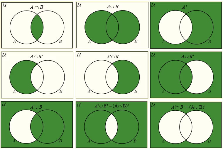
Complementary Events

For any event E, the complementary event not E is the event that E does not occur.
The probability of the complementary event is: $P (\neg E) = 1 - P (E)$
Example: If the probability of raining tomorrow is 0.3, then the probability that it does not rain is: 1-0.3=0.71

Continuous Probability

Continuous probability deals with events that have an infinite number of possible outcomes, like measuring time, height, or temperature.
In continuous probability, the outcomes are not distinct (like heads or tails) but can take any value in a given range. We don't calculate probabilities for specific values, but instead for ranges of values.

Why is Probability Important?

It helps us make decisions when we don't know what will happen.
It is the foundation for statistics, data science, and machine learning.

How is Statistics and Probability connected?

Statistics helps interpret the results of testing machine learning models and make better decisions
Probability provides the foundation for understanding statistics and its tools.

II. The Rules (Axioms) of Probability

These forms the foundation for calculating and understanding probabilities.

Img Src: https://fiveable.me

These are the basic rules that all probabilities must follow:

Non-Negativity:
- The probability of any event E is always between 0 and 1 (inclusive).
- There are no events that can have negative probability. $0 \leq P (E) \leq 1$
Total Probability:
- The probability of the entire sample space S, which includes all possible outcomes, is always 1.
- This means something in the sample space is guaranteed to happen. $P (S) = 1$
Additivity:
- If two events cannot happen at the same time (mutually exclusive), then $P (A or B) = P (A) + P (B)$
- Example: When flipping a coin, getting heads and getting tails are mutually exclusive. $P (H or T) = 1$

III. Approaches to Probability

There are three main ways to think about probability:

Axiomatic Probability (based on rules/axioms)
Frequentist Probability (based on experiments and data)
Classical Probability (based on equally likely outcomes)

★ Axiomatic Probability

Uses the three rules above to define probability for any situation.
Example: If Anna watches drama 40% of the time and action 30% of the time, the chance she watches either is $0.4 + 0.3 = 0.7$ .

★ Frequentist Probability

Based on experiments or data. Probability is the long-run frequency of an event.
Example: Anna watched 12 dramas out of 30 movies last year. Probability she picks a drama next is $12 / 30 = 0.4$ .

★ Classical Probability

All outcomes are equally likely. Probability is just "favorable outcomes divided by total outcomes."
Example: Anna has 4 dramas out of 10 movies. Probability she picks a drama is $4 / 10 = 0.4$ .

ASPECT	FREQUENTIST PROBABILITY	CLASSICAL PROBABILITY
Definition	Probability is defined as the long-run relative frequency of an event occurring in repeated trials.	Probability is based on the assumption that all outcomes in the sample space are equally likely.
Interpretation	Probability is an empirical measure derived from repeated experiments.	Probability is derived theoretically based on symmetry and logical reasoning.
Assumption	Assumes an infinite number of trials for probabilities to converge.	Assumes all possible outcomes have the same likelihood.
Calculation	Estimated from observed frequencies over repeated trials.	Computed using the formula: P(A) = (Favorable outcomes) / (Total outcomes)
Example	If a coin is flipped 1,000 times and lands on heads 520 times, the probability of heads is estimated as 520/1000 = 0.52.	The probability of getting heads in a fair coin toss is 1/2 since both outcomes are equally likely.
Alignment with Axioms	Follows the Axioms of Probability but interprets probability through empirical observations.	Fully adheres to Axiomatic Probability, assuming equal likelihood of all outcomes.

4. Counting Principles: How Many Ways?

To find the probability of an event, we first need to count the number of outcomes. Counting plays a key role in determining the size of the sample space and calculating probabilities. By knowing how many ways an event can happen, we can better understand its likelihood.

There are two fundamental rules for counting:

1. The Addition Rule (for "OR")

If you have two events are mutually exclusive (you can't pick both), you add the number of options.
Example: If you can take a bus (3 routes) OR a train (2 routes) to school, you have $3 + 2 = 5$ total ways to get there.

2. The Multiplication Rule (for "AND")

If you have to make a sequence of choices, you multiply the number of options at each step.
Example: To create an outfit, you choose from 3 shirts AND 2 pairs of pants. You have $3 \times 2 = 6$ possible outfits.

I. Types of Counting

Based on the multiplication rule, we can handle more complex scenarios. The key questions to ask are: "Does order matter?" and "Can I reuse items?"

★ Exponents (Counting with Replacement)

Use exponents when you are making a sequence of choices from the same set of options, and you can pick the same option more than once.
Here repetitions are allowed.
Formula: $n^{r}$ , where $n$ is the number of options for each choice, and $r$ is the number of choices you make.
Example: A 3-digit lock can use digits from 0-9. How many combinations are possible?
- You have 10 choices for the first digit, 10 for the second, and 10 for the third.
- Total combinations = $10 \times 10 \times 10 = 10^{3} = 1000$ .

★ Factorials (Counting without Replacement)

If repetitions are not allowed, the number of available options decreases with each selection, and we use factorials.
A factorial is the product of all integers from $1$ to $n$ .
Example: For a padlock where you choose a 4-digit password from combo from 10 numbers without repeats,
- The number of combinations is: $10 \times 9 \times 8 \times 7 = 5040$

★ Permutations (Order Matters, Without Replacement)

Use permutations when you are arranging a set of items, and you cannot reuse an item. The order of arrangement is important.
Formula: $P (n, r) = \frac{n!}{(n - r)!}$
- Where $n$ is the total number of items, and $r$ is how many you choose to arrange.
Example: How many ways can you award 1st, 2nd, and 3rd place to 8 runners?
- Order matters (1st is different from 2nd). You can't give one runner two prizes.
- $P (8, 3) = \frac{8!}{(8 - 3)!} = \frac{8!}{5!} = 8 \times 7 \times 6 = 336$ ways.

★ Combinations (Order Does NOT Matter, Without Replacement)

a.k.a Binomial Coefficients
Use combinations when you are selecting a group of items, and the order of selection does not matter.
Formula: $C (n, r) = (\binom{n}{r}) = \frac{n!}{r! (n - r)!}$
- Where $n$ is the total number of items, and $r$ is how many you choose.
Example: How many ways can you choose 3 students out of 5 to form a committee?
- Order doesn't matter (a committee of Alice, Bob, and Charlie is the same as Charlie, Alice, and Bob).
- $C (5, 3) = \frac{5!}{3! (5 - 3)!} = \frac{5!}{3! 2!} = \frac{120}{6 \times 2} = 10$ ways.

II. The Inclusion-Exclusion Principle

What if events are NOT mutually exclusive? If we just add them, we double-count the overlap. The inclusion-exclusion principle helps us correct this.
The Inclusion-Exclusion Principle helps calculate the probability of the union of overlapping events by subtracting the over-counted intersections.

Formula for two events:

\begin{aligned} P (A or B) & = P (A) + P (B) - P (A and B) \\ P (A \cup B) & = P (A) + P (B) - P (A \cap B) \end{aligned}

We subtract the intersection ( $A \cap B$ ) to remove the double-counted outcomes.

Example:
In a class of 30 students, 15 play soccer, 10 play basketball, and 5 play both. What is the probability that a randomly chosen student plays soccer or basketball?

Let S be the event "plays soccer" and B be "plays basketball."
$P (S) = 15 / 30 = 0.5$
$P (B) = 10 / 30 \approx 0.33$
$P (S and B) = 5 / 30 \approx 0.17$
$P (S or B) = P (S) + P (B) - P (S and B) = 0.5 + 0.33 - 0.17 = 0.66$ .
So, there is a 66% chance a student plays at least one of the sports.

V. Advanced Probability Concepts

1. Independent Events:

Two events are independent if knowing one happened does NOT change the chance of the other.
Mathematically:
- Independent Events: $P (A \cap B) = P (A) \cdot P (B)$
- Dependent Events:
Example: Flipping a coin twice. Getting heads the first time doesn't affect the second flip.

2. Mutually Exclusive Events:

Two events are mutually exclusive if they cannot both happen at the same time.
Mathematically: $P (A \cap B) = 0$
Example: Rolling a die, getting a 1 and getting a 2 are mutually exclusive.

3. Comparison Example:

Let A = {roll a 6}, B = {roll a 2 or 3} on a die.

$P (A) = 1 / 6$ , $P (B) = 1 / 3$
$P (A \cap B) = 0$ (they can't both happen)
$P (A) \cdot P (B) = 1 / 18 \neq 0$
So, A and B are mutually exclusive, but NOT independent.

Case study

Simple case: Rolling a fair die, let Event A = {roll a 6} and let B =

$P (A) = \frac{1}{6}$
$P (B) = \frac{1}{3}$
$P (A and B) = P (A \cap B) = 0$
$P (A or B) = P (A \cup B) = \frac{1}{2}$

Question: Are the events Independent, Mutually exclusive or neither?

As per the definition of Independence $P (A \cap B) = P (A) . P (B)$

$P (A) \cdot P (B) = \frac{1}{6} \cdot \frac{1}{3} = \frac{1}{18} \neq 0$
$∴$ Events A and B are NOT independent

As per definition of Mutual Exclusive $P (A \cup B) = P (A) + P (B) - P (A \cap B)$

$P (A) + P (B) - P (A \cap B) = \frac{1}{6} + \frac{1}{3} - 0 = \frac{1}{2} = \frac{1}{2}$
$∴$ the events are mutually exclusive

VI. Conditional Probability

Conditional probability is the chance that something happens, given that something else has already happened.
Formula:

P (A | B) = \frac{P (A \cap B)}{P (B)}

Example:
If 30% of students play football, and 10% play both football and basketball, then the probability a student plays basketball given they play football is $P (B | F) = \frac{0.10}{0.30} = 0.33$ .

Note

P (A \cap B) = P (A | B) P (B) = P (B | A) P (A)

This becomes the basis of Naive Bayes Theorem

Bayes' Theorem:
This is a special formula for "flipping" conditional probabilities:

VII. Partition and The Law of Total Probability

Sometimes, it's hard to calculate the probability of an event directly. The Law of Total Probability gives us a clever way to find it by breaking the problem into smaller, easier pieces.

★ What is a Partition?

A partition is a way of dividing the entire sample space into several events that are:

Mutually Exclusive: None of the events overlap.
Exhaustive: Together, the events cover all possible outcomes.

Think of it like slicing a pizza. Each slice is a separate piece (mutually exclusive), and all the slices together make up the whole pizza (exhaustive).

Simple Example: For tomorrow's weather, the events "Rain" and "No Rain" form a partition. They can't both happen, and one of them must happen.

★ The Law of Total Probability

This law states that you can find the probability of an event (let's call it A) by considering how it behaves within each piece of the partition.

Formula: If $B_{1}, B_{2}, . . ., B_{n}$ form a partition of the sample space, then for any event A:

P (A) = P (A | B_{1}) P (B_{1}) + P (A | B_{2}) P (B_{2}) + . . . + P (A | B_{n}) P (B_{n})

In simple terms: The total probability of A is a weighted average of its conditional probabilities, where the weights are the probabilities of each event in the partition.

Example 1: Choosing a Marble

Imagine two bags of marbles.

Bag 1: Contains 3 red and 7 blue marbles.
Bag 2: Contains 6 red and 4 blue marbles.

You flip a fair coin to decide which bag to draw from. What is the probability you pick a red marble?

Event A: Picking a red marble.
Partition: The choice of bag. Let $B_{1}$ be "choose Bag 1" and $B_{2}$ be "choose Bag 2".
- $P (B_{1}) = 0.5$ (from the coin flip)
- $P (B_{2}) = 0.5$ (from the coin flip)
Conditional Probabilities:
- The probability of getting red given you chose Bag 1 is $P (A | B_{1}) = 3 / 10 = 0.3$ .
- The probability of getting red given you chose Bag 2 is $P (A | B_{2}) = 6 / 10 = 0.6$ .
Total Probability:
- $P (A) = P (A | B_{1}) P (B_{1}) + P (A | B_{2}) P (B_{2})$
- $P (A) = (0.3 \times 0.5) + (0.6 \times 0.5) = 0.15 + 0.30 = 0.45$

So, the overall probability of picking a red marble is 45%.

Example 2: Student Study Habits

At a school, students are either "Full-Time" or "Part-Time".

60% of students are Full-Time ( $P (F T) = 0.6$ ).
40% are Part-Time ( $P (P T) = 0.4$ ).

We also know:

50% of Full-Time students study on weekends ( $P (Weekend | F T) = 0.5$ ).
80% of Part-Time students study on weekends ( $P (Weekend | P T) = 0.8$ ).

What is the probability that a randomly chosen student studies on the weekend?

Event A: A student studies on the weekend.
Partition: Student status, "Full-Time" (FT) and "Part-Time" (PT).
Total Probability:
- $P (A) = P (A | F T) P (F T) + P (A | P T) P (P T)$
- $P (A) = (0.5 \times 0.6) + (0.8 \times 0.4) = 0.30 + 0.32 = 0.62$

So, there is a 62% chance that any given student studies on the weekend. This law is a key ingredient in Bayes' Theorem.

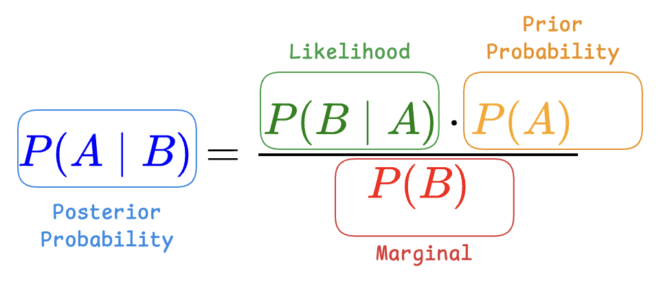
VIII. Bayes' Theorem (Putting It All Together)

Bayes' theorem helps us update our beliefs when we get new information. It connects conditional probabilities in a powerful way.

Formula:

P (A ∣ B) = \frac{P (B ∣ A) \cdot P (A)}{P (B)}

Key Terms:

Prior Probability ( $P (A)$ ):
- What you believed about A before seeing new evidence B.
- Example: Suppose 5% of the population has a certain disease. Before testing, your prior belief about someone having the disease is 5%.
Likelihood ( $P (B | A)$ ):
- How likely is the evidence B if your belief A is true?
- Example: A medical test correctly identifies the disease 99% of the time (i.e., if someone has the disease, the test will be positive 99% of the time).
Posterior Probability ( $P (A | B)$ ):
- What you should believe about A after seeing the evidence B.
Marginal Likelihood ( $P (B)$ ):
- The overall probability of observing the evidence B. This is often calculated using the Law of Total Probability!

Example: The "Positive Test" Problem Revisited

Suppose 1% of people have a certain disease. A test for it is 99% accurate for sick people, but has a 2% false positive rate (healthy people who test positive). If you test positive, what is the chance you actually have the disease?

Step 1: Define Events

$D$ : You have the disease.
$H$ : You are healthy.
$T^{+}$ : You test positive.

Step 2: List the Probabilities

Prior: $P (D) = 0.01$ . So, $P (H) = 1 - 0.01 = 0.99$ .
Likelihoods:
- $P (T^{+} | D) = 0.99$ (A sick person tests positive).
- $P (T^{+} | H) = 0.02$ (A healthy person tests positive).

Step 3: Calculate $P (T^{+})$ using the Law of Total Probability
The sample space is partitioned into "Disease" and "Healthy".

$P (T^{+}) = P (T^{+} | D) P (D) + P (T^{+} | H) P (H)$
$P (T^{+}) = (0.99 \times 0.01) + (0.02 \times 0.99) = 0.0099 + 0.0198 = 0.0297$
The overall chance of anyone testing positive is about 3%.

Step 4: Apply Bayes' Theorem
We want to find $P (D | T^{+})$ , the probability of having the disease given a positive test.

$P (D | T^{+}) = \frac{P (T^{+} | D) \cdot P (D)}{P (T^{+})}$
$P (D | T^{+}) = \frac{0.99 \times 0.01}{0.0297} \approx 0.333$

So, even with a positive test, the chance you have the disease is only about 33.3%! This surprising result happens because the disease is rare.

Example 2: The Defective Bolt Problem

In a factory, three machines, $M_{1}$ , $M_{2}$ , and $M_{3}$ , produce 2000, 2500, and 4000 bolts daily, respectively. Their defect rates are:

Machine $M_{1}$ : 3%
Machine $M_{2}$ : 4%
Machine $M_{3}$ : 2.5%

A bolt is drawn randomly from a day's production and found to be defective. What is the probability it was produced by machine $M_{2}$ ?

Step 1: Define Events

$M_{1}$ : The bolt is from machine $M_{1}$ .
$M_{2}$ : The bolt is from machine $M_{2}$ .
$M_{3}$ : The bolt is from machine $M_{3}$ .
$D$ : The bolt is defective.

We want to find $P (M_{2} | D)$ .

Step 2: List the Probabilities
First, let's find the prior probabilities of a bolt coming from each machine.

Total bolts produced = $2000 + 2500 + 4000 = 8500$ .
$P (M_{1}) = 2000 / 8500 \approx 0.235$
$P (M_{2}) = 2500 / 8500 \approx 0.294$
$P (M_{3}) = 4000 / 8500 \approx 0.471$

Next, list the likelihoods (the defect rates for each machine).

$P (D | M_{1}) = 0.03$
$P (D | M_{2}) = 0.04$
$P (D | M_{3}) = 0.025$

Step 3: Calculate P(D) using the Law of Total Probability
The events $M_{1}$ , $M_{2}$ , and $M_{3}$ form a partition of the sample space.

$P (D) = P (D | M_{1}) P (M_{1}) + P (D | M_{2}) P (M_{2}) + P (D | M_{3}) P (M_{3})$
$P (D) = (0.03 \times 0.235) + (0.04 \times 0.294) + (0.025 \times 0.471)$
$P (D) \approx 0.00705 + 0.01176 + 0.011775 \approx 0.030585$

The overall probability of picking a defective bolt is about 3.06%.

Step 4: Apply Bayes' Theorem
Now we can calculate the posterior probability, $P (M_{2} | D)$ .

$P (M_{2} | D) = \frac{P (D | M_{2}) \cdot P (M_{2})}{P (D)}$
$P (M_{2} | D) \approx \frac{0.04 \times 0.294}{0.030585} \approx \frac{0.01176}{0.030585} \approx 0.3845$

Conclusion:
The probability that the defective bolt came from machine $M_{2}$ is approximately 38.5%.

Why is Bayes' Theorem Important?

It provides a mathematical way to update our beliefs in light of new evidence.
It is the foundation of many machine learning algorithms (like Naive Bayes classifiers), medical diagnostic tools, and spam filters.

IX. Key Takeaways

Probability is about reasoning with uncertainty. It gives us a framework to make logical decisions when we don't have all the facts.
Always define your sample space and events clearly. This is the most important step in solving any probability problem.
Counting is key. Use the right tool for the job: the addition rule for "OR" choices, and the multiplication rule (exponents, permutations, combinations) for "AND" sequences.
Don't double-count. Use the inclusion-exclusion principle when events can happen at the same time.
Context matters. Conditional probability ( $P (A | B)$ ) is one of the most important ideas. It's the probability of A, in the new world where we know B has happened.
Update your beliefs. The Law of Total Probability and Bayes' Theorem are powerful tools for breaking down complex problems and updating our knowledge as we get new data.