Gaussian Distribution (Normal Distribution)

The Normal distribution, also called the Gaussian distribution, is the most important distribution in statistics and machine learning.

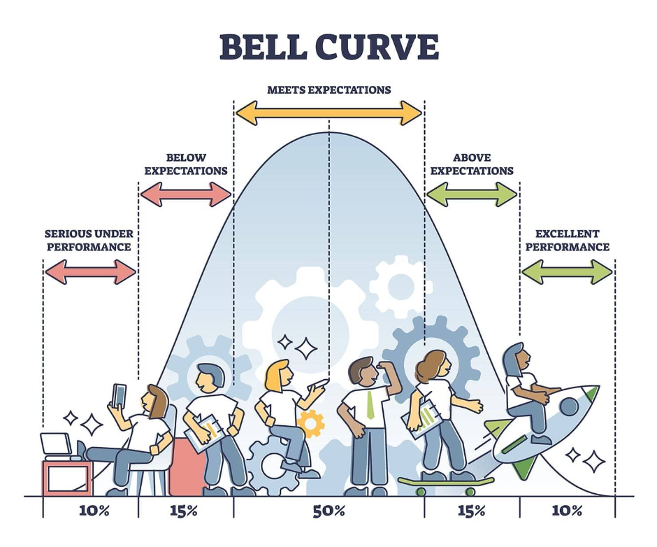
We all would have heard, during our yearly performance review that management has adjusted your rating to fit in a belt curve. Below is that bell curve. 🤣 —this is the shape of the normal distribution!

1. What is the Normal Distribution?

A normal distribution is a continuous probability distribution that is symmetric about its mean, showing that data near the mean are more frequent in occurrence than data far from the mean. In graph form, the normal distribution will appear as a bell curve.

2. Key Properties

• Random Variable ($X$): Can take any real value from $-\mathrm{\infty }$ to $+\mathrm{\infty }$.
• Symmetry: The distribution is perfectly symmetric about the mean.
• Parameters:
  • Mean ($\mu$): The center of the distribution (also the median and mode).
  • Variance (${\sigma }^2$): Measures the spread of the distribution.
  • Standard Deviation ($\sigma$): The square root of the variance.
• Probability Density Function (PDF):$$f(x;\mu ,\sigma )=\frac{1}{\sigma \sqrt{2\pi }}{e}^{-\frac{(x-\mu {)}^2}{2{\sigma }^2}},-\mathrm{\infty }<x<+\mathrm{\infty }$$

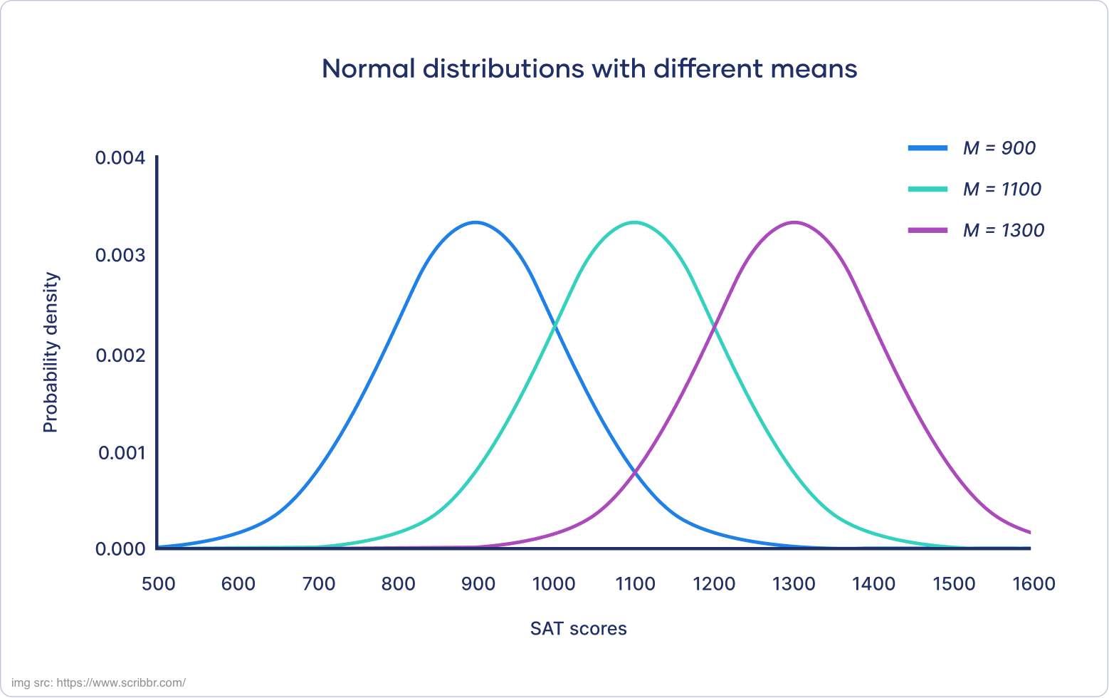
3. Visualizing the Parameters

• Mean ($\mu$): Determines the location of the peak (center) of the curve.

  • Increasing $\mu$ shifts the curve to the right.
  • Decreasing $\mu$ shifts the curve to the left.
    

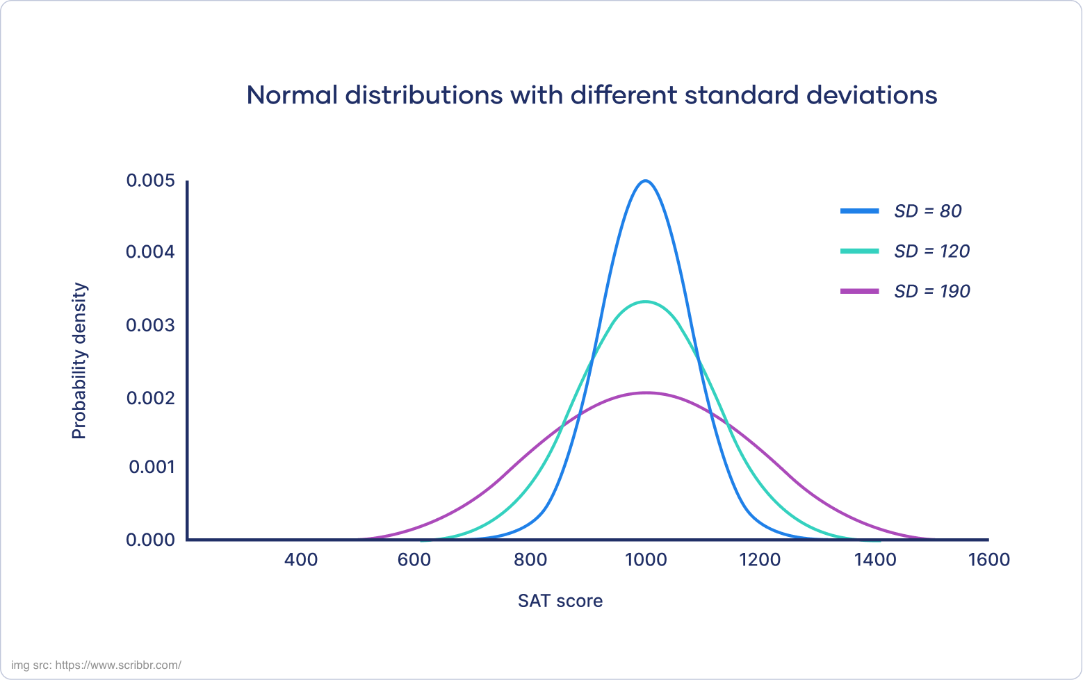
• Standard Deviation ($\sigma$): Controls the width (spread) of the curve.

  • Small $\sigma$: Narrow, tall curve.
  • Large $\sigma$: Wide, flat curve.
    

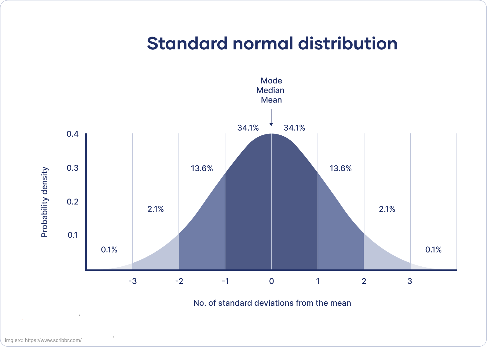
4. The Empirical Rule (68-95-99.7 Rule)

This rule tells us how data is distributed in a normal distribution:

• 68% of values fall within 1 standard deviation of the mean.
• 95% of values fall within 2 standard deviations of the mean.
• 99.7% of values fall within 3 standard deviations of the mean.

5. Standard Normal Distribution

The standard normal distribution is a special case where:

• $\mu =0$
• $\sigma =1$
• The random variable is called $Z$.

The PDF becomes:

where $z=\frac{x-\mu }{\sigma }$ is called the z-score.

6. Example: Heights of Students

Suppose the heights of students in a school are normally distributed with a mean ($\mu$) of 170 cm and a standard deviation ($\sigma$) of 10 cm.

(a) What is the probability that a randomly chosen student is taller than 185 cm?

Step 1: Convert to z-score

Step 2: Find the probability using the standard normal table

• $P(X>185)=P(Z>1.5)$
• From the z-table, $P(Z<1.5)\approx 0.9332$
• So, $P(Z>1.5)=1-0.9332=0.0668$

Final Answer:
There is a 6.68% chance that a randomly chosen student is taller than 185 cm.

(b) What percentage of students are between 160 cm and 180 cm?

Step 1: Convert both values to z-scores

• For 160 cm: $z_1=\frac{160-170}{10}=-1$
• For 180 cm: $z_2=\frac{180-170}{10}=1$

Step 2: Find probabilities from the z-table

• $P(Z<1)\approx 0.8413$
• $P(Z<-1)\approx 0.1587$

Step 3: Subtract to find the probability between

Final Answer:
About 68.26% of students are between 160 cm and 180 cm tall.