Continuous Probability Distributions

Recap: Probability Distribution

A probability distribution is a function or rule that describes how probability is spread across the possible values of a random variable.

I. What is a Continuous Probability Distribution?

A continuous probability distribution describes the probabilities of a continuous random variable $X$ —one that can take any value within a range ‒ which can be infinite, and therefore uncountable. Examples include height, weight, or time.

II. Probability Density Function (PDF)

Since there are infinite possible values, we use a Probability Density Function (PDF) to describe the distribution.

★ Defination

The probability density function(PDF) is the function that represents the density of probability for a continuous random variable over the specified ranges.

🤔 Unlike a PMF, the value of the PDF at a specific point, $f (x)$ , is not the probability of that point. It is the density.

★ Key Formulas

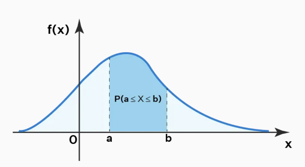
Probability Density Function (PDF): $f (x)$ , gives the density of probability at each value of $x$ . Probability is represented by area under the curve. The probability that $X$ falls within an interval $[a, b]$ is the area under the curve between $a$ and $b$ : $$\large P(a \leq X \leq b) = \int_{a}^{b} f(x) , dx$$
Cumulative Distribution Function (CDF): Calculates the area under the curve up to a certain point, representing the cumulative probability.

F (x) = P (X \leq x) = \int_{- \infty}^{x} f (t) d t

Mean: ( $E [X]$ or $μ$ ) represents the "center of mass" or the long-term average of the distribution.

E [X] = \int_{- \infty}^{\infty} x f (x) d x

Variance: ( $V a r (X)$ or $σ^{2}$ ) measures the "spread" of the data around the mean. It is the average of the squared deviations from the mean.

V a r (X) = \int_{- \infty}^{\infty} x^{2} f (x) d x

★ Key properties

Non-negativity: The function can never be negative. You can't have a "negative density."

f (x) \geq 0 for all x

Total area under the PDF curve is 1: The entire area under the curve and above the x-axis equals 1, representing 100% certainty that the variable will take a value within its possible range. $$\large \displaystyle \int^{\infty}_{-\infty} f(x) , dx = 1$$
Probability of any exact value is zero: Since a continuous variable can take an infinite number of values within a range, the probability of it taking any specific single value is mathematically zero.$$P(X = a) = 0$$
Outcomes are measured, not counted: Continuous variables represent measurable quantities like time, weight, or temperature, which can take any value within a given interval.
The graph is a smooth curve: The distribution is visualized as a continuous, smooth curve rather than discrete bars.

★ Example: Waiting for a Bus (Uniform Distribution)

Scenario:
You arrive at a bus stop where a bus arrives every 20 minutes, but you don't know when the last one left. Your waiting time, $X$ , is a random variable between 0 and 20 minutes.

Random Variable ( $X$ ): The time (in minutes) you wait for the next bus.
Possible Values: $0 \leq X \leq 20$
Since every arrival time is equally likely, this follows a Continuous Uniform Distribution. To ensure the total area equals 1 over a 20-minute span, the "height" (density) of the function must be $1 / 20$ .
PDF $f (x)$ : $$
f(x) = \left{
\begin{array} \
\frac{1}{20} & \mbox{if } 0 \le x \le 20 \
0 & \mbox{otherwise} \
\end{array}\right.

- * * Q u e s t i o n : * * W h a t i s t h e p r o b a b i l i t y y o u w a i t b e t w e e n 5 a n d 10 m i n u t e s ? - * * S t e p 1 : S e t u p t h e i n t e g r a l * *

P(5 \leq X \leq 10) = \int_{5}^{10} \frac{1}{20} dx

- * * S t e p 2 : C a l c u l a t e t h e a r e a * * W e f i n d t h e a r e a o f t h e r e c t a n g l e b e t w e e n $ x = 5 $ a n d $ x = 10 $ . $ $ P (5 \leq X \leq 10) = \int_{5}^{10} \frac{1}{20} d x = \frac{1}{20} (10 - 5) = 0.25

Result: There is a 25% chance your wait time falls in that 5-minute window.

III. Common Continuous Distributions

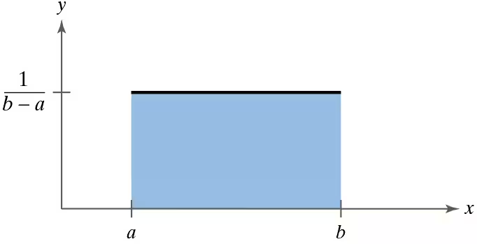
1. Uniform Distribution

The Uniform distribution is the simplest continuous distribution. Every value in a specified range is equally likely.

Key properties

The Random Variable:
- A random variable is distributed uniformly is written as $X \sim U (a, b)$
- $X$ can take any value in the interval $[a, b]$ .
  - $a$ : the minimum value (lower bound).
  - $b$ : the maximum value (upper bound).
Height: The height of the PDF is constant between a and b.
Normality: The total area under the curve (which represents the total probability) is 1.
Probability Density Function (PDF): $f (x) = {\begin{cases} \frac{1}{b - a} & a \leq x \leq b \\ 0 & otherwise \end{cases}$
Cumulative Distribution Function (CDF):

F (X) = \frac{x - a}{b - a} where a \leq x \leq b

Mean: $μ_{x} = E (X) = \frac{a + b}{2}$
Variance: $σ^{2} = \frac{(b - a)^{2}}{12}$
Example:
A random number generator produces numbers uniformly between 0 and 10. What is the probability of getting a number between 3 and 7?

P (3 \leq X \leq 7) = \int_{3}^{7} \frac{1}{10} d x = \frac{1}{10} \times (7 - 3) = 0.4

2. Normal (Gaussian) Distribution

Definition: The most important distribution in statistics and machine learning. Many natural phenomena (like heights, test scores) follow this distribution.
PDF: $f (x; μ, σ) = \frac{1}{σ \sqrt{2 π}} e^{- \frac{(x - μ)^{2}}{2 σ^{2}}}$ where $μ$ is the mean and $σ$ is the standard deviation.
Read Gaussian Distribution for details.

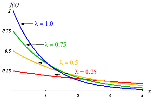
3. Exponential Distribution

The Exponential Distribution is a continuous probability distribution that models the time or space between independent events occurring at a constant average rate, such as customer arrivals, radioactive decay, or machine failures. It is highly skewed, with small values being more frequent than large ones.

Formulas

The Parameter: $λ$ (lambda): Rate parameter (average number of events per unit time)
The Random Variable: $X \geq 0$ (time or distance).
Probability Density Function (PDF): $f (x; λ) = {\begin{cases} λ e^{- λ x} & x \geq 0 \\ 0 & x < 0 \end{cases}$
Cumulative Distribution Function (CDF):

F (x) = 1 - e^{- λ x} for x \geq 0

Mean = Median = $\frac{1}{λ}$
Variance = $\frac{1}{λ^{2}}$

Key properties

Modeling Time-to-Event: It measures "how long until the next event".
Relationship to Poisson: If events follow a Poisson Distribution (number of events in a set time), the time between those events follows an exponential distribution.
Shape: It is a right-skewed distribution, often starting at 0 and descending gradually
Memoryless Property: The probability of an event occurring in the next $x$ minutes is independent of how much time has already passed. $$P(X > s + t \mid X > s) = P(X > t)$$

Example:
Average time between customers is 5 minutes ( $λ = 0.2$ per minute).
Probability next customer arrives within 3 minutes:

P (X \leq 3) = 1 - e^{- 0.2 \times 3} = 1 - e^{- 0.6} \approx 0.451

Questions and Answers

Q1: What is the difference between the Poisson distribution and exponential distribution?
Poisson distribution deals with the number of occurrences of events in a fixed period of time, whereas the exponential distribution is a continuous probability distribution that often concerns the amount of time until some specific event happens.

Q2: Why is the exponential distribution memoryless?
The key property of the exponential distribution is memoryless as the past has no impact on its future event's occurance, and each instant is like the starting of the new random period.

Q3: What does lambda mean in the exponential distribution?
The lambda in exponential distribution represents the rate parameter, and it defines the mean number of events in an interval.

$λ$ indicates how quickly the decay of the exponential function occurs.
Changing the decay parameter affects how fast the probability distribution converges to zero.
As $λ$ increases, the distribution decays faster, i.e, we obtain a steeper curve.

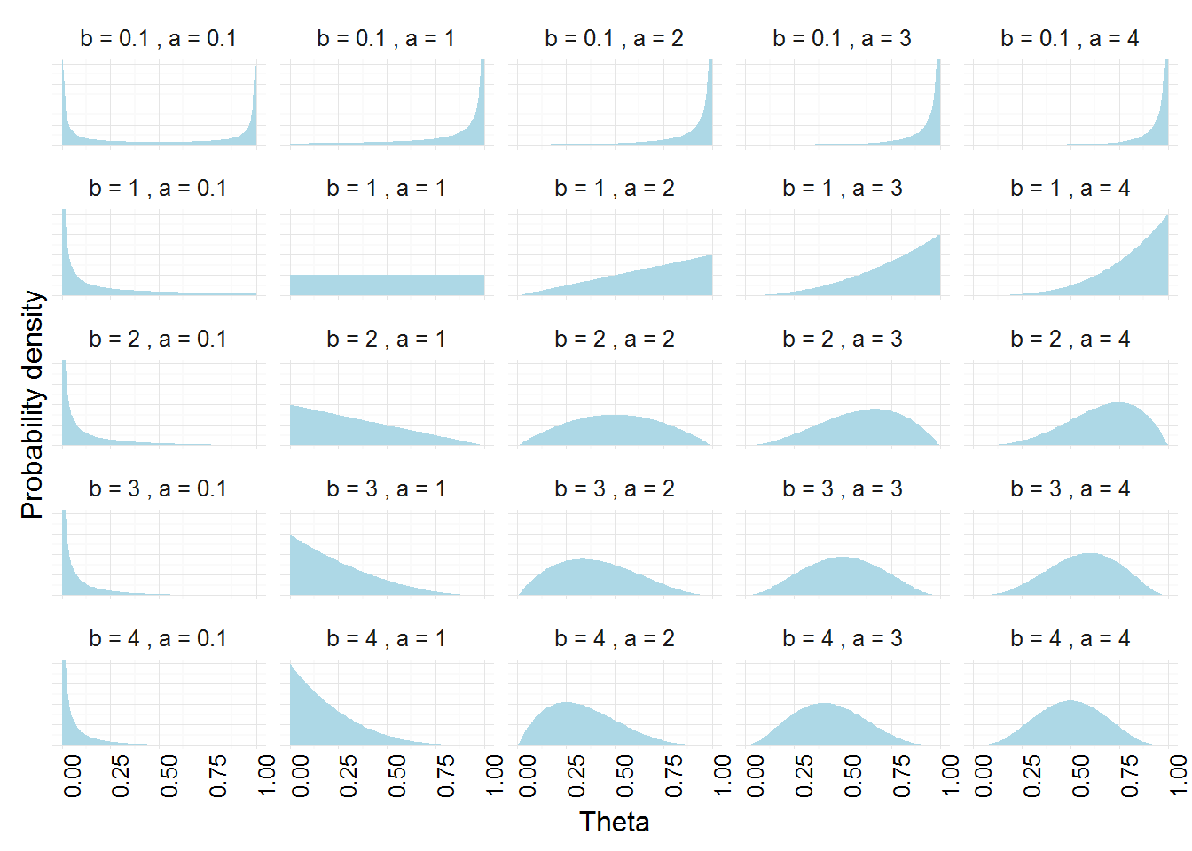
4. Beta Distribution (Advanced)

The Beta distribution is a continuous probability distribution often used to model the uncertainty about the probability of success of an experiment.
The Beta distribution can be used to analyze probabilistic experiments that have only two possible outcomes:

success, with probability
failure, with probability
These experiments are called Bernoulli experiments.

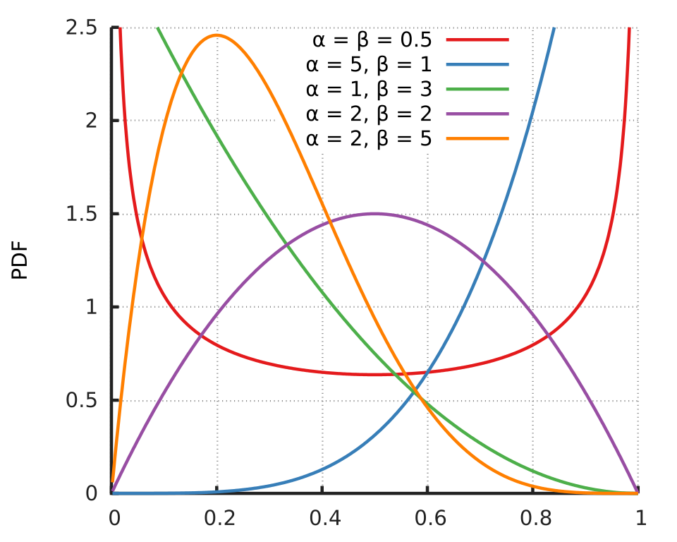
Key Properties and Formulas

Domain: [0,1] ➛ Models probabilities themselves (values between 0 and 1)
PDF:
$f (x; α, β) = \frac{1}{B (α, β)} x^{α - 1} (1 - x)^{β - 1}$
where $B (α, β)$ is the beta function, which ensures the total probability integrates to 1, and $α, β > 0$ .
Mean = $\frac{α}{α + β}$
Variance: $\frac{α β}{(α + β)^{2} (α + β + 1)}$
Shape: Can take various shapes depending on $α$ and $β$
- $α$ = 1, $β$ = 1 ➛ Uniform Distribution
- $α$ , $β$ < 1 ➛ U-Shaped Distribution
- $α$ , $β$ > 1 ➛ The distribution is unimodal (one peak).
- $α$ = $β$ ➛ Symmetric
- $α$ < $β$ ➛ the distribution is skewed right.
- $α$ > $β$ ➛ the distribution is left right.
Concentration:
- Increasing both $α$ and $β$ , increases the concentration of the distribution around the mean, representing greater certainty (narrower distribution)
- Larger value of $α$ , higher likelihood concentrating density toward 1.
- Larger value of $β$ , higher likelihood concentrating density toward 0

Binomial vs Beta

	BINOMIAL DISTRIBUTION	BETA DISTRIBUTION
Purpose	Models the number of successes in a fixed number of trials.	Models the probability of success in a probabilistic experiment.
Usecase	Used when the probability of success is known and fixed	Used when the probability of success is uncertain
Outcome	Discrete distribution where outcomes are numbers	Continuous distribution where outcomes lie in [0,1]
Formula	$$f(x) = \binom{n}{k}; p^k (1-p)^{n-k}$$ $w h e r e f (x) i s f u n c t i o n o f x$	$$g(p) = \frac{1}{B(\alpha, \beta)} ; p^{\alpha-1} (1-p)^{\beta-1}$$ $w h e r e g (p) i s f u n c t i o n o f p$