I. Entropy 》II. Joint Entropy 》III. Conditional Entropy 》IV. Mutual Information 》V. Information Gain

III. Conditional Entropy and Weighted Entropy

1. What is Conditional Entropy $H (Y | X)$ ?

★ Core Concept: If Shannon Entropy $H (Y)$ is the "total surprise" in $Y$ , then Conditional Entropy $H (Y | X)$ is the "leftover surprise" once you know the value of $X$ .

★ Real-World Example:
In a Decision Tree context: "On average, how confused am I about whether someone will play golf once I know the weather?"

★ Key Property:

One-sided relationship: We care about predicting $Y$ , and $X$ is just additional information to help us.

★ General Interpretation:

Conditional entropy of $Y$ given $X$ is the remaining entropy of $Y$ when $X$ is fixed
It represents the part of the entropy of $Y$ that is uninformative about $X$
Also called the "noise entropy" of $Y$ with respect to $X$

Key Properties and Boundary Cases

Condition	Mathematical Statement	Interpretation	Practical Meaning
Reduction Property	$H (Y ∣ X) \leq H (Y)$	Knowing $X$ can only reduce (or maintain) uncertainty in $Y$	Information never hurts!
Perfect Predictor	$H (Y ∣ X) = 0$	$Y$ is a deterministic function of $X$	No uncertainty remains; $X$ perfectly predicts $Y$
Strong Predictor	$H (Y ∣ X) \approx 0$	Very low remaining uncertainty	$X$ is an excellent feature for predicting $Y$
Complete Independence	$H (Y ∣ X) = H (Y)$	$X$ and $Y$ are independent	Knowing $X$ provides zero information about $Y$
Weak Predictor	$H (Y ∣ X) \approx H (Y)$	High remaining uncertainty	$X$ is a useless feature for predicting $Y$

Rule of Thumb for Feature Evaluation

$H (Y | X)$ close to 0 → Feature $X$ is a very strong predictor of $Y$ ✅
$H (Y | X)$ moderately low → Feature $X$ is somewhat useful in predicting $Y$ ⚠️
$H (Y | X)$ close to $H (Y)$ → Feature $X$ is useless ❌

2. Mathematical Foundation

★ Formula

H (Y | X) = \sum_{x \in X} P (x) \cdot H (Y | X = x)

This is the conditional entropy of $Y$ given $X$ . It measures the average remaining uncertainty in $Y$ once you know the value of $X$ .

Alternative (Expanded) Form:

H (Y | X) = - \sum_{x \in X} \sum_{y \in Y} P (x, y) \log_{2} P (y | x)

★ Understanding the Components

$X$ and $Y$ : discrete random variables
$x \in X$ : loop over all possible values that variable $X$ can take
$y \in Y$ : loop over all possible values that variable $Y$ can take
$P (x)$ : probability that $X = x$ (proportion of data where feature equals $x$ )
$P (y ∣ x)$ : conditional probability that $Y = y$ given $X = x$
$P (x, y)$ : joint probability that $X = x$ and $Y = y$
$H (Y | X = x)$ : entropy of $Y$ within the specific subset where $X = x$
$\log_{2} P (y ∣ x)$ : logarithm base 2, so entropy is measured in bits
Negative sign: makes the result non-negative (since $\log_{2} P (y ∣ x) \leq 0$ )

3. Interpreting Conditional Entropy Values

Conditional entropy of Y (given X) is the remaining entropy of Y when X is fixed. Thus, conditional entropy of Y (given X) is the part of the entropy of Y that is uninformative about X. For this reason, it is also called the ‘noise entropy’ of A (with respect to B)
Reduction: $H (Y | X) \leq H (Y)$ . Knowing $X$ can only reduce or maintain the uncertainty of $Y$ ; it can never increase it.
Independence: If $X$ and $Y$ are completely independent, then $H (Y | X) = H (Y)$ (knowing $X$ helps zero percent).
Perfect Correlation: If $Y$ is a deterministic function of $X$ , then $H (Y | X) = 0$ (no uncertainty remains).
If $H (Y | X)$ is close to 0: The feature $X$ is a very strong predictor. Most of the uncertainty is gone.
If $H (Y | X)$ is close to 1: The feature $X$ is USELESS.
If $H (Y | X)$ is close to $H (Y)$ : The feature $X$ is useless. Knowing $X$ didn't help you predict $Y$ at all.

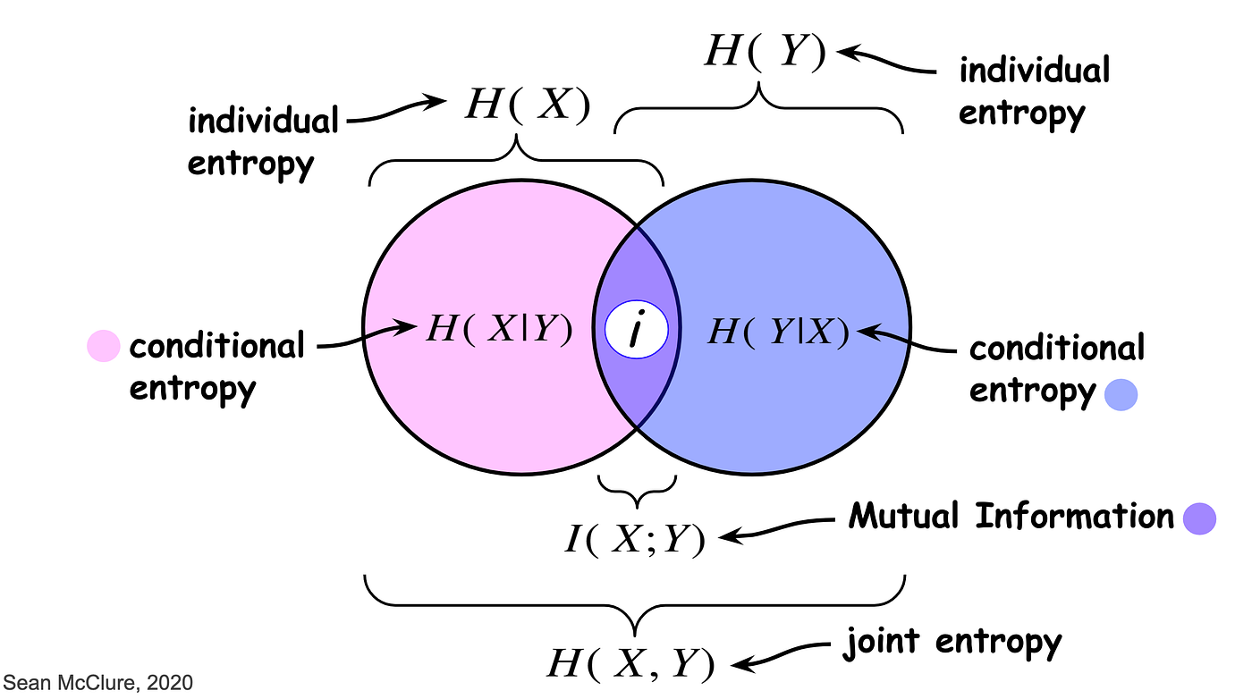
4. Relationship to Other Entropy Measures

★ Chain Rule for Entropy

The joint, conditional, and marginal entropies are related as follows:

H (X, Y) = H (X | Y) + H (Y) = H (Y | X) + H (X)

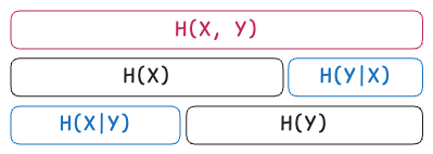
In words: The joint entropy of $X$ and $Y$ equals the conditional entropy of $X$ given $Y$ , plus the marginal entropy of $Y$ (and vice-versa).

Rearranging for Conditional Entropy:

\begin{aligned} H (Y | X) & = H (X, Y) - H (X) & \dots (Equation 1) \\ H (X | Y) & = H (X, Y) - H (Y) & \dots (Equation 2) \end{aligned}

Interpretation: Conditional Entropy is the difference between the total system uncertainty (joint entropy) and the uncertainty of the known variable.

★ Derivation of the Chain Rule

\begin{aligned} H (X, Y) & = - \sum_{x \in X} \sum_{y \in Y} P (x, y) \log_{2} P (x, y) \\ Apply Product Rule: P (x, y) = P (x) P (y | x) \\ H (X, Y) & = - \sum_{x \in X} \sum_{y \in Y} P (x, y) \log_{2} (P (x) P (y | x)) \\ Use Log Property: \log (A B) = \log A + \log B \\ H (X, Y) & = - [\sum_{x \in X} \sum_{y \in Y} P (x, y) \log_{2} P (x) + \sum_{x \in X} \sum_{y \in Y} P (x, y) \log_{2} P (y | x)] \\ Simplify the first term using Marginal Probability: \sum_{y} P (x, y) = P (x) \\ H (X, Y) & = - [\sum_{x \in X} P (x) \log_{2} P (x) + \sum_{x \in X} \sum_{y \in Y} P (x, y) \log_{2} P (y | x)] \\ Recognize that - \sum P (x) \log_{2} P (x) = H (X) \\ H (X, Y) & = H (X) + [- \sum_{x \in X} \sum_{y \in Y} P (x) P (y | x) \log_{2} P (y | x)] \\ Move P (x) outside the inner sum over y : \\ H (X, Y) & = H (X) + \sum_{x \in X} P (x) (- \sum_{y \in Y} P (y | x) \log_{2} P (y | x)) \\ Recognize the inner sum as the entropy of a specific branch: H (Y | X = x) \\ H (X, Y) & = H (X) + \sum_{x \in X} P (x) \cdot H (Y | X = x) \\ Final Identity: \\ H (X, Y) & = H (X) + H (Y | X) \end{aligned}

Key Takeaway

Conditional Entropy accounts for relationships between variables and is mathematically linked through the Chain Rule of Information:

$H (X, Y)$ : The Joint Entropy (total uncertainty of the combined system)
$H (X)$ : The Shannon Entropy of the predictor variable $X$
$H (Y | X)$ : The Conditional Entropy (remaining uncertainty about $Y$ after knowing $X$ )

5. Weighted Entropy

★ Understanding the Name "Weighted Entropy"

Weighted Entropy is another name for Conditional Entropy, but it emphasizes the computational perspective—how we actually calculate it in practice, especially when building decision trees or selecting features.

Key Insight: Two Names, One Concept

Conditional Entropy and Weighted Entropy refer to the same concept:

Conditional Entropy is the theoretical name: "entropy of $Y$ given $X$ "
Weighted Entropy is the practical name: "weighted average of subset entropies"

They produce identical numerical results!

★ Why "Weighted"?

When we split data using feature $X$ , we create subsets (branches). Each subset has its own entropy, but they don't all matter equally—larger subsets should have more influence on the final metric.

The Weighted Average Formula:

H (Y | X) = \sum_{x \in X} P (x) \cdot H (Y | X = x)

Breaking it down:

$P (x)$ : The weight — the proportion of samples in subset $x$
$H (Y | X = x)$ : The entropy of the target $Y$ within subset $x$
We multiply each subset's entropy by its proportion (weight), then sum them up

Example: Unfair Split

Imagine splitting 100 patients into two groups:

Group A (Fever): 90 patients with mixed outcomes (entropy = 0.9 bits)
Group B (No Fever): 10 patients, all perfectly classified (entropy = 0 bits)

❌ Without weighting (WRONG):

Simple Average = (0.9 + 0.0) / 2 = 0.45 bits

This makes the split look excellent because Group B is perfect, but Group B only represents 10% of the data!

✅ With weighting (CORRECT):

Weighted Average = (0.9 × 0.9) + (0.1 × 0.0) = 0.81 bits

Interpretation: Even though Group B is perfect, the overall weighted entropy is 0.81 because 90% of the data is still messy. The split provided 0.19 bits of information gain (1.0 - 0.81), which is modest.

Comparison Table: Weighted vs Unweighted

Scenario	Unweighted Average	Weighted Average	Why Weighted is Better
Balanced split Group A: 50 samples, entropy = 0.8 Group B: 50 samples, entropy = 0.6	$(0.8 + 0.6) / 2 = 0.7$	$(0.5 \times 0.8) + (0.5 \times 0.6) = 0.7$	Same result—no bias when balanced
Imbalanced split Group A: 90 samples, entropy = 0.9 Group B: 10 samples, entropy = 0.1	$(0.9 + 0.1) / 2 = 0.5$ ❌	$(0.9 \times 0.9) + (0.1 \times 0.1) = 0.82$ ✅	Correctly reflects that most data is still messy
Extreme imbalance Group A: 99 samples, entropy = 1.0 Group B: 1 sample, entropy = 0.0	$(1.0 + 0.0) / 2 = 0.5$ ❌	$(0.99 \times 1.0) + (0.01 \times 0.0) = 0.99$ ✅	Prevents tiny pure groups from dominating

6. Step-by-Step Calculation: A Complete Example

The Dataset: Flu Diagnosis

Let's use the same flu example with a concrete dataset:

Given:

10 patients total
Target Y (Flu): 6 have Flu, 4 don't
Feature X (Fever): 7 have Fever, 3 don't

Data Table:

Fever (X)	Flu (Y)	Count
Yes	Yes	5
Yes	No	2
No	Yes	1
No	No	2

Step 1: Split by Feature X (Create Subsets)

Subset 1 (Fever = Yes): 7 patients (5 with flu, 2 without)
Subset 2 (Fever = No): 3 patients (1 with flu, 2 without)

Step 2: Calculate Entropy for Each Subset

Subset 1 Entropy (Fever = Yes):

H (Y | X = Yes) = - (\frac{5}{7} \log_{2} \frac{5}{7} + \frac{2}{7} \log_{2} \frac{2}{7}) = 0.863 bits

Subset 2 Entropy (Fever = No):

H (Y | X = No) = - (\frac{1}{3} \log_{2} \frac{1}{3} + \frac{2}{3} \log_{2} \frac{2}{3}) = 0.918 bits

Step 3: Calculate Weights (Proportions)

Weight for Subset 1: $P (X = Yes) = 7 / 10 = 0.7$
Weight for Subset 2: $P (X = No) = 3 / 10 = 0.3$

Step 4: Compute Weighted Average

\begin{aligned} H (Y | X) & = P (X = Yes) \times H (Y | X = Yes) + P (X = No) \times H (Y | X = No) \\ = (0.7 \times 0.863) + (0.3 \times 0.918) \\ = 0.604 + 0.275 \\ = 0.879 bits \end{aligned}

Step 5: Interpret the Result

What does 0.879 bits mean?

On average, after knowing if a patient has a fever, you still have 0.879 bits of uncertainty about whether they have the flu
The feature "Fever" reduced uncertainty, but not dramatically

Calculate Information Gain:
First, we need the original total entropy:

H (Y) = - (\frac{6}{10} \log_{2} \frac{6}{10} + \frac{4}{10} \log_{2} \frac{4}{10}) = 0.971 bits

Then:

Information Gain = H (Y) - H (Y | X) = 0.971 - 0.879 = 0.092 bits

Conclusion: Since the Information Gain is positive (but small), "Fever" is a somewhat helpful feature, but it hasn't completely resolved the uncertainty. The decision tree might need additional features to improve prediction.

7. Machine Learning Applications

1. How Decision Tree Algorithms Use Weighted Entropy

When a decision tree algorithm (like ID3, C4.5, or CART) evaluates a potential split, it follows these exact steps:

Algorithm Steps:

Calculate weighted entropy for every possible feature
Compare them to find which gives the lowest weighted entropy
Choose that feature for splitting (because it gives the highest Information Gain)
Repeat recursively for each branch until stopping criteria are met

Python Implementation

def weighted_entropy(data, feature, target):
    """
    Calculate weighted entropy for a split on 'feature'
    
    Parameters:
    - data: DataFrame containing the dataset
    - feature: Name of the feature column to split on
    - target: Name of the target column
    
    Returns:
    - Weighted entropy (float)
    """
    total_entropy = 0
    total_samples = len(data)
    
    # For each unique value of the feature
    for feature_value in data[feature].unique():
        # Create subset where feature == feature_value
        subset = data[data[feature] == feature_value]
        
        # Calculate weight (proportion of data in this subset)
        weight = len(subset) / total_samples
        
        # Calculate entropy of target within this subset
        subset_entropy = calculate_entropy(subset[target])
        
        # Add weighted contribution
        total_entropy += weight * subset_entropy
    
    return total_entropy

2. Feature Selection Process

Example: Comparing Multiple Features

Feature: "Patient ID is odd/even" (Bad Feature)
- Group A (Odd): 5 patients, entropy = 0.97 bits (still random)
- Group B (Even): 5 patients, entropy = 0.97 bits (still random)
Weighted Entropy = (0.5 × 0.97) + (0.5 × 0.97) = 0.97 bits
Information Gain = 0.97 - 0.97 = 0 bits
→ Feature REJECTED! ❌

Feature: "Temperature > 38°C" (Good Feature)
- Group A (High temp): 6 patients, entropy = 0.65 bits (mostly sick)
- Group B (Normal temp): 4 patients, entropy = 0.81 bits (mostly healthy)
Weighted Entropy = (0.6 × 0.65) + (0.4 × 0.81) = 0.714 bits
Information Gain = 0.97 - 0.714 = 0.256 bits
→ Feature SELECTED! ✅

The algorithm chooses "Temperature" because it has higher Information Gain.

8. Summary and Key Takeaways

Essential Points to Remember

1. Conditional Entropy = Weighted Entropy

Same concept, different names
"Conditional" emphasizes theory; "Weighted" emphasizes computation

2. The Formula

H (Y | X) = \sum_{x \in X} P (x) \cdot H (Y | X = x)

$P (x)$ = weight (proportion of data in subset $x$ )
$H (Y | X = x)$ = entropy within subset $x$

3. Why Weighting Matters

Larger subsets have more influence (correctly!)
Prevents tiny pure groups from dominating
Essential for fair feature comparison

4. Relationship to Information Gain

Information Gain = H (Y) - H (Y | X)

Higher gain = better feature
Decision trees maximize information gain at each split

5. Used in Every Major Algorithm

ID3, C4.5, CART
Random Forest, XGBoost, Gradient Boosting
Any tree-based method for classification

Quick Reference Guide

When evaluating a feature split:

✅ Calculate entropy for each subset: $H (Y | X = x)$
✅ Weight by subset size: $P (x) = n_{x} / n_{total}$
✅ Sum weighted contributions: $H (Y | X) = \sum P (x) \cdot H (Y | X = x)$
✅ Compare to original entropy: $IG = H (Y) - H (Y | X)$
✅ Choose feature with highest Information Gain

Interpretation shortcuts:

$H (Y | X) \approx 0$ → Excellent feature! Strong predictor
$H (Y | X) \approx 0.5 \times H (Y)$ → Decent feature, provides some information
$H (Y | X) \approx H (Y)$ → Useless feature, provides no information

Key Insight: Conditional Entropy = Weighted Entropy

Conditional Entropy and Weighted Entropy are the same concept:
- Conditional Entropy is the theoretical definition: $H (Y | X) = H (X, Y) - H (X)$
- Weighted Entropy is the practical computation: $H (Y | X) = \sum P (x) \cdot H (Y | X = x)$

Both give you the same result—they're just different perspectives on calculating "uncertainty remaining after knowing X."