Understanding the ANOVA Test Results

How comparing “between” vs “within” variation tells us if group means truly differ?

Introduction

Imagine five classrooms, each trying a different study technique. At the end of the term, every student takes the same exam. You look at the average score in each class and wonder: Are these teaching methods really different, or are the average differences just random wiggles?

That question is exactly what ANOVA (Analysis of Variance) answers. ANOVA is a way to compare three or more group means by asking a simple-but-powerful question: Is the variation between group averages big compared to the natural variation within each group?

If “between” variation dwarfs “within” variation, at least one group mean is likely different. If not, the differences you see are probably just noise.

What ANOVA Tests?

Null hypothesis ( $H_{0}$ ): All groups have the same mean.
Alternative hypothesis ( $H_{a}$ ): At least one group has a significantly different mean.
Big picture: How unusual is our data if H0 were true? ANOVA turns this into a single test statistic called F.

The F-statistic and p-value are derived from an Analysis of Variance (ANOVA) test, which compares the means of multiple groups to determine if at least one group is significantly different.

How ANOVA Works in Feature Selection: A Flowchart

START: Select a numerical feature (e.g., 'study_hours') and a categorical target (e.g., 'result')

I: Group Data:

Split the dataset into groups based on each category of the target variable.(e.g., Group 1: 'Pass', Group 2: 'Fail')

II: Calculate Variances

Calculate Variance BETWEEN groups (Signal)
Calculate Variance WITHIN each group (Noise)

III: Compute F-Statistic

Calculate the ratio of between-group variance to within-group variance.

IV: Determine Statistical Significance

Calculate the p-value associated with the F-statistic.
(A small p-value, typically < 0.05, means the result is statistically significant).

V: Rank and Select Features Repeat for all numerical features

Rank them by their F-values (higher is better).
Select the top-k features for your model.

Understanding the ANOVA Test Results

I had always been wondering the math behind Anova testing, which is one to be used for feature selection when we have Continuous Dependent Variable and Categorical Target Variable. Thus my attempt is to shot the math behind using the one example.

Sample data for this example is picked up from scipy’s documentation’s, f_oneway, which performs one-way ANOVA tests.

Tillamook (10 values) = $(0.0571, 0.0813, 0.0831, 0.0976, 0.0817, 0.0859, 0.0735, 0.0659, 0.0923, 0.08360)$
Newport (8 values) = $(0.0873, 0.0662, 0.0672, 0.0819, 0.0749, 0.0649, 0.0835, 0.0725)$
Petersburg (7 values) = $(0.0974, 0.1352, 0.0817, 0.1016, 0.0968, 0.1064, 0.105)$
Magadan (8 values) = $(0.1033, 0.0915, 0.0781, 0.0685, 0.0677, 0.0697, 0.0764, 0.0689)$
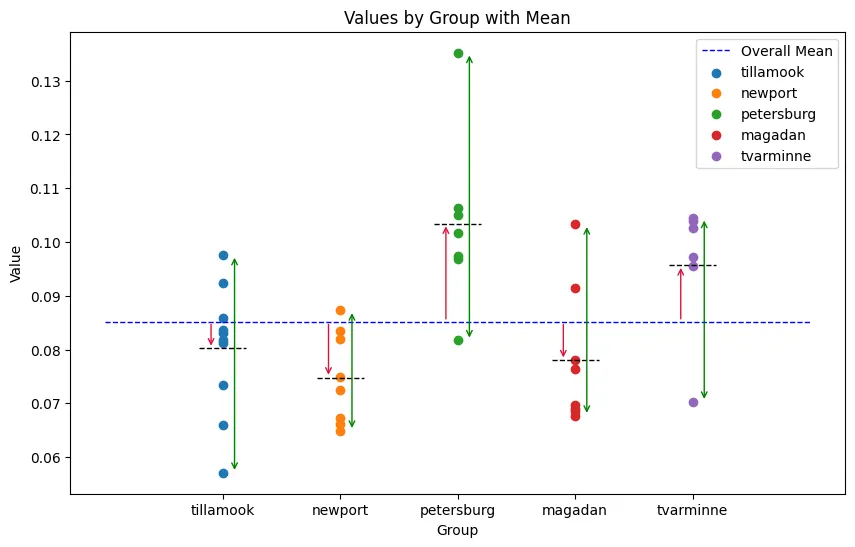
Tvarminne (6 values) = $(0.0703, 0.1026, 0.0956, 0.0973, 0.1039, 0.1045)$

In above graph each group mean as a black dash on a line. Blue dashed line plots the grand mean. The red arrows from each grand mean to the group mean show “between-group” difference. If the null is true (all means equal), those arrows should be tiny. Green dash line represents the variance in each group.

ANOVA asks: Are the red arrows (between) meaningfully bigger than the green arrows (within)? If yes, the groups likely have different means.?

F-statistic Formula

F = \frac{Between-group variance}{Within-group variance} ​ = \frac{M S_{b e t w e e n}}{M S_{w i t h i n}}

Where:

Between-group variance ( $M S_{b e t w e e n}$ ): Measures variability between different groups
Within-group variance ( $M S_{w i t h i n}$ ): Measures variability within each group

★ Step 1: General Stats

Number of Groups (k) and Total Observations (N):
- k=5 (Tillamook, Newport, Petersburg, Magadan, Tvarminne)
- N=39 (Total number of observations)
- $X i j$ is $i^{t h}$ data point in group $j$

★ Step 2: Compute Mean

i. First, we calculate the mean ( $\bar{x}$ ) for each group (location).

Tillamook ( $n_{1} = 10$ ): $\sum X_{T i l l a m o o k} = 0.802$ , ${\bar{x}}_{1} = 0.0802$
Magadan ( $n_{4} = 8$ ): $\sum X_{M a g a d a n} = 0.5951$ , ${\bar{x}}_{4} = 0.0744$
Tvarminne ( $n_{5} = 6$ ): $\sum X_{T v a r m i n n e} = 0.5742$ , ${\bar{x}}_{5} = 0.0957$
Petersburg ( $n_{3} = 7$ ): $\sum X_{P e t e r s b u r g} = 0.7241$ , ${\bar{x}}_{3} = 0.1034$
Newport ( $n_{2} = 8$ ) : $\sum X_{N e w p o r t} = 0.5984$ , ${\bar{x}}_{2} = 0.0748$

ii. Grand Mean ( ${\bar{X}}_{G}$ ):**

\begin{array}{r} {\bar{X}}_{G} = \frac{\sum_{i} \sum_{j} X_{i j}}{N} = 0.0845 \end{array}

★ Step 3: Compute Sum of Squares

i. Sum of Squares Between Groups ( $S S_{b e t w e e n}$ )

\begin{aligned} S S_{b e t w e e n} & = \sum n_{i} (\bar{X_{i}} - G M)^{2} \\ = 10 \cdot (0.080 - 0.0852)^{2} + 8 \cdot (0.075 - 0.0852) + 7 \cdot (0.103 - 0.0852) + 8 \cdot (0.078 - 0.0852) + 6 \cdot (0.096 - 0.0852) \\ = 0.00025 + 0.00087 + 0.00233 + 0.00041 + 0.00066 \\ S S_{b e t w e e n} & = 0.00452 \end{aligned}

Where $n_{i}$ is the number of observations in each group, $\bar{X_{i}}$ is the mean of each group.

ii. Sum of Squares Within Groups ( $S S_{w i t h i n}$ )

This measures the "noise" or spread inside each individual group. We find the sum of squared differences from each group's own mean.

Tillamook: $\sum (x - 0.0802)^{2} = 0.00025$
Petersburg: $\sum (x - 0.1034)^{2} = 0.00233$
Magadan: $\sum (x - 0.0744)^{2} = 0.00041$
Tvarminne: $\sum (x - 0.0957)^{2} = 0.00066$
Newport: $\sum (x - 0.0748)^{2} = 0.00087$

\begin{aligned} S S_{w i t h i n} & = \sum \sum (X_{i j} - \bar{X_{i})^{2}} \\ S S_{w i t h i n} & = 0.00539 \end{aligned}

iii. Total Sum of Squares ( $S S_{t o t a l}$ )

\begin{aligned} S S_{t o t a l} & = S S_{b e t w e e n} + S S_{w i t h i n} \\ = 0.00452 + 0.00539 \\ = 0.00991 \end{aligned}

★ Step 4: Compute Mean Squares

Degrees of Freedom

$d f_{b e t w e e n} = (Groups - 1) = (5 - 1) = 4$
$d f_{w i t h i n} = (Total Samples - Groups) = (39 - 5) = 34$
Between-group variance ( $M S_{b e t w e e n}$ ): Measures variability between different groups

M S_{b e t w e e n} = \frac{S S_{b e t w e e n}}{d f_{b e t w e e n}} = \frac{0.00452}{4} = 0.00113

Within-group variance ( $M S_{w i t h i n}$ ): Measures variability within each group

M S_{w i t h i n} = \frac{S S_{w i t h i n}}{d f_{w i t h i n}} = \frac{0.00539}{39} = 0.000159

★ Step 5: Compute the F-Statistic

The F-statistic is calculated as:

\begin{aligned} F & = \frac{Between-group variance}{Within-group variance} ​ & = \frac{M S_{b e t w e e n}}{M S_{w i t h i n}} = \frac{0.00113}{0.000159} \\ = 7.12101947164245 \end{aligned}

★ Step 6: (Final) p-value calculation

Once we compute the F-statistic, the p-value is obtained from the F-distribution:

p-value = Probability of getting an F-statistic this extreme under the null hypothesis
If p-value < α (0.05), reject $H_{0}$ (at least one group is significantly different)
If p-value > α (0.05), fail to reject $H_{0}$ (no significant difference)

Final Interpretation

In our case when $F = 7.121$ , $p = 0.00028$
Since p < 0.05, we reject the null hypothesis, meaning at least one group has a significantly different mean.

Interpreting Common Scenarios

Low between-group variance, any within-group variance: Groups look similar. F small. Fail to reject H0.
High between-group variance, low within-group variance: Clear separation. F very large. Reject H0.
Unequal within-group variances across groups: Violates a key ANOVA assumption. Consider Welch’s ANOVA or nonparametric alternatives.
High between-group variance, high within-group variance: Means differ, but overlap makes it harder. F may or may not be large. You need the ANOVA to decide.

Python Code

import numpy as np  
from scipy.stats import f_oneway  
  
tillamook = [0.0571, 0.0813, 0.0831, 0.0976, 0.0817, 0.0859, 0.0735, 0.0659, 0.0923, 0.0836]  
newport = [0.0873, 0.0662, 0.0672, 0.0819, 0.0749, 0.0649, 0.0835, 0.0725]  
petersburg = [0.0974, 0.1352, 0.0817, 0.1016, 0.0968, 0.1064, 0.105]  
magadan = [0.1033, 0.0915, 0.0781, 0.0685, 0.0677, 0.0697, 0.0764, 0.0689]  
tvarminne = [0.0703, 0.1026, 0.0956, 0.0973, 0.1039, 0.1045]  
  
f_oneway(tillamook, newport, petersburg, magadan, tvarminne)

Output

F_onewayResult(statistic=np.float64(7.121019471642445), pvalue=np.float64(0.00028122423145345525))

Understanding the ANOVA Test Results

Introduction

What ANOVA Tests?

How ANOVA Works in Feature Selection: A Flowchart

Understanding the ANOVA Test Results

F-statistic Formula

★ Step 1: General Stats

★ Step 2: Compute Mean

i. First, we calculate the mean (x¯) for each group (location).

ii. Grand Mean (X¯G):**

★ Step 3: Compute Sum of Squares

i. Sum of Squares Between Groups (SSbetween)

ii. Sum of Squares Within Groups (SSwithin)

iii. Total Sum of Squares (SStotal)

★ Step 4: Compute Mean Squares

Degrees of Freedom

★ Step 5: Compute the F-Statistic

★ Step 6: (Final) p-value calculation

Interpreting Common Scenarios

Python Code

i. First, we calculate the mean ( $\bar{x}$ ) for each group (location).

ii. Grand Mean ( ${\bar{X}}_{G}$ ):**

i. Sum of Squares Between Groups ( $S S_{b e t w e e n}$ )

ii. Sum of Squares Within Groups ( $S S_{w i t h i n}$ )

iii. Total Sum of Squares ( $S S_{t o t a l}$ )