Mean Squared Logarithmic Error (MSLE)

Definition

Mean squared logarithmic (MSLE) is a regression loss function that measures the average squared difference between the logarithms of predicted and actual values and provides a better measure of the relative errors between the two values

MSLE is a less commonly used loss function.

MSLE measures the ratio between true and predicted values by taking the log of both before calculating the squared error. This makes it particularly useful when you care about relative errors rather than absolute errors, or when your target variable spans several orders of magnitude.

Formula:

M S L E = \frac{1}{n} \sum_{i = 1}^{n} (\log (y_{i} + 1) - \log (\hat{y_{i}} + 1))^{2}

The "+1" is added to handle cases where Actual target value ( $y$ ) or Predicted value ( $\hat{y}$ ) might be zero.

Advantages

1. Handles Large-Scale Variations (Multi-Order Magnitude Robustness)

Works well when target values span multiple orders of magnitude (e.g., 1, 100, 10,000, 100,000).
Perfect for exponential data: Population counts, sales volumes, viral growth, housing prices, etc.
Scale compression: The log transformation compresses large values, preventing them from dominating the loss.
Example: Predicting population—errors on cities (millions) and towns (thousands) are treated proportionally.
Analogy: Like using a logarithmic scale on a graph—you can see trends from 1 to 1,000,000 without the large values crushing the small ones.

2. Treats Relative Errors Equally (Percentage-Aware Loss)

A 10% error on a value of 100 is weighted the same as a 10% error on a value of 1000.
Mathematical property: $\log (110 / 100) = \log (1100 / 1000)$ — same relative change, same log difference.
Fair comparison: Unlike MSE where a $100 error on $1000 is penalized 100x less than a $100 error on $100.
Business alignment: Often mirrors how we think—being 10% off is 10% off, regardless of the absolute value.
Impact: Model focuses on improving relative accuracy across all scales, not just on large values.

3. Robustness to Outliers (Log Compression Effect)

Less sensitive to extreme outliers compared to Mean Squared Error (MSE).
Why: Taking the log before squaring compresses the range and prevents massive values from dominating.
Example: An outlier at 1,000,000 becomes log(1,000,000) ≈ 13.8, which is much more manageable.
Comparison: MSE would square the raw error, MSLE squares the log of the ratio.
When it helps: Financial data with occasional extreme values, web traffic with viral spikes.

4. Penalizes Underprediction More (Asymmetric by Design)

Underpredicting is penalized more heavily than overpredicting by the same percentage.
Mathematical reason: Log function is concave—underprediction creates larger log differences.
Example:
- Actual = 100, Predicted = 50 (50% under) → log error ≈ 0.69
- Actual = 100, Predicted = 150 (50% over) → log error ≈ 0.41
Use case: Inventory management, capacity planning—better to overestimate than underestimate and run out of stock.
Impact: Model naturally learns to be more conservative, avoiding severe underpredictions.

Disadvantages

1. Only Works with Non-Negative Values (Log Domain Restriction)

Cannot handle negative target values—you can't take the log of a negative number.
Fatal limitation: If your target can be negative (e.g., profit/loss, temperature changes), MSLE is unusable.
Zero handling: The "+1" in the formula is a workaround, but it's not perfect for data that naturally includes zeros.
Impact: Limits applicability to specific domains—counts, prices, populations, etc.
The Fix: Use alternatives like RMSLE (Root MSLE) with careful zero handling, or choose a different loss if negatives are present.

2. Asymmetric Penalty (Underprediction Bias)

Under-predictions are penalized more heavily than over-predictions of the same magnitude.
Mathematical asymmetry: $\log (90 / 100) \neq \log (110 / 100)$ in magnitude—the first is larger.
Concrete example:
- Actual = 100, Predicted = 80 (20% under) → MSLE contribution ≈ 0.0506
- Actual = 100, Predicted = 120 (20% over) → MSLE contribution ≈ 0.0297
- Underprediction penalized ~1.7x more!
Impact: Models trained with MSLE tend to overpredict to avoid the heavier penalty.
When problematic: If overprediction has serious consequences (e.g., overordering inventory with expiration dates), MSLE may not align with business objectives.

3. Harder to Interpret (Log-Scale Abstraction)

The loss is in log-scale, making it less intuitive than MAE or RMSE.
Communication challenge: "MSLE = 0.05" doesn't immediately tell you how far off your predictions are in original units.
Not directly comparable: You can't say "we improved from MSLE 0.10 to 0.05, so we're twice as good."
Stakeholder confusion: Business users prefer "we're off by $100 on average" (MAE) over "our log-squared error is 0.5."
The Fix: Convert to RMSLE (take square root) or report supplementary metrics like MAE/MAPE alongside MSLE.

4. Sensitive to Small Values (The "+1" Problem)

Adding 1 to handle zeros can distort the loss for very small true values.
Why it's problematic:
- Actual = 0.01, Predicted = 0.02 → With "+1": $\log (1.01) - \log (1.02)$ ≈ tiny difference
- The "+1" dominates for small values, masking the 100% error!
Example: If your data ranges from 0.001 to 0.1, the "+1" makes everything close to 1, losing sensitivity.
Impact: MSLE works best when target values are >= 1. For fractional data, it may not behave as expected.
The Fix: Consider using log1p with appropriate scaling, or ensure your target values are in a range where "+1" is negligible.

When to Use MSLE

Your target variable has exponential growth or spans multiple orders of magnitude (e.g., prices, populations, counts)
You care about percentage errors rather than absolute errors
Underprediction is worse than overprediction (e.g., forecasting demand - better to overestimate than run out of stock)
All target values are non-negative

Scaling and Practical Considerations

1. Does MSLE Need Scaled Data?

The short answer: Feature scaling helps, but target scaling is problematic.
The real answer: MSLE has unique scaling properties because it already applies log transformation to the target, which is itself a form of scaling.

2. Key Insight: MSLE Already Transforms the Target

The critical difference from other losses:

MSLE applies $\log (y + 1)$ and $\log (\hat{y} + 1)$ , which compresses the range of values.
This log transformation is a non-linear scaling operation built into the loss function.
Implication: Adding additional target scaling on top of log transformation can distort the relative error interpretation.

What the log does:

Converts multiplicative relationships to additive ones
Compresses large values more than small values
Makes the metric focus on relative (percentage) errors rather than absolute errors

Analogy: MSLE is like a camera with a built-in filter. Adding another filter (scaling) might improve some aspects but can also create unexpected distortions.

3. When does scaling help?

★ Feature Scaling - Recommended

Scale features for model training, not for MSLE

Gradient-based models (Neural Networks, SGD):

Feature scaling improves convergence speed and training stability.
Different feature scales can cause inconsistent gradient magnitudes.
Impact: Same benefits as with MSE—faster, more stable optimization.

Regularized models (Ridge, Lasso):

Essential for fair regularization across all features.
Without scaling, regularization penalizes coefficients based on feature units, not importance.
Analogy: Regularization is a "tax" on coefficients—scaling ensures the tax is fair.

Neural networks:

Critical for proper weight initialization and activation function behavior.
Prevents vanishing/exploding gradients caused by scale mismatches.

Multi-feature models:

Ensures all features contribute based on predictive power, not numeric range.
Example: House prices with "square footage" (1000-5000) and "bedrooms" (1-10)—square footage would dominate without scaling.

4. Why Target Scaling is NOT Recommended for MSLE

The core issue: MSLE already handles wide value ranges through its built-in log transformation.

Problem 1: Double transformation creates distortion

# Original: Actual = 100, Predicted = 110 (10% error)
# MSLE = (log(101) - log(111))^2 ≈ 0.0091

# After standardization (mean=1000, std=500):
# Scaled actual = -1.8, Scaled predicted = -1.78
# Can't compute log of negative numbers! MSLE breaks completely.

Problem 2: MinMax scaling changes relative errors

# Original values: 10, 100, 1000
# Log differences capture relative changes correctly

# After MinMax (0-1): 0.01, 0.10, 1.0
# Log(1.01) - Log(1.10) ≈ 0.085
# vs
# Log(11) - Log(101) ≈ 2.22 (original scale)
# The relative error interpretation is lost!

Problem 3: Loses the "relative percentage error" property

The whole point of MSLE is to treat 10% error equally whether the value is 100 or 1000.
Target scaling breaks this property because it changes the relative relationships between values.

5. Effect of Scaling on MSLE

Scaling Type	Effect on MSLE	Recommendation
Feature Scaling Only	No effect on MSLE; improves model training	✅ Highly Recommended
Target StandardScaler	Creates negative values → log fails or produces nonsense	❌ Never use
Target MinMax (0-1)	Distorts relative error interpretation; changes MSLE values unpredictably	❌ Don't use
Target Log Transform	Redundant—MSLE already does this; use MSE instead if you pre-transform	⚠️ Use MSE on log-transformed target instead
No target scaling	MSLE works as designed	✅ Best for MSLE

6. MSLE vs. Manual Log Transform: What's the Difference?

Two equivalent approaches:

Approach 1: Use MSLE with original target

# Model predicts original scale
model.fit(X_train_scaled, y_train)  # y_train in original scale
y_pred = model.predict(X_test_scaled)

# Calculate MSLE (log happens inside the metric)
from sklearn.metrics import mean_squared_log_error
msle = mean_squared_log_error(y_test, y_pred)

Approach 2: Manual log transform + MSE

# Transform target manually
y_train_log = np.log1p(y_train)  # log(y + 1)
y_test_log = np.log1p(y_test)

# Model predicts log scale
model.fit(X_train_scaled, y_train_log)
y_pred_log = model.predict(X_test_scaled)

# Calculate MSE on log scale (equivalent to MSLE)
from sklearn.metrics import mean_squared_error
mse_log = mean_squared_error(y_test_log, y_pred_log)  # This equals MSLE!

# Transform predictions back to original scale
y_pred = np.expm1(y_pred_log)  # exp(y_pred_log) - 1

Which to choose?

Approach 1: Simpler code, model predicts in original units (easier to interpret)
Approach 2: More flexible—you can use any loss function (MSE, MAE, Huber) on log scale
Both produce the same result mathematically!

7. Best Practice for MSLE

✅ Always standardize FEATURES for better model training:

from sklearn.preprocessing import StandardScaler

scaler_X = StandardScaler()
X_train_scaled = scaler_X.fit_transform(X_train)
X_test_scaled = scaler_X.transform(X_test)

❌ NEVER scale the TARGET when using MSLE as your metric

✅ Ensure non-negative values:

# Clip predictions to be non-negative
y_pred = np.maximum(y_pred, 0)

# Or handle at prediction time
y_pred = model.predict(X_test)
y_pred = np.clip(y_pred, 0, None)

💡 Alternative: Log transform manually and use MSE:

# Transform target
y_train_log = np.log1p(y_train)

# Train on log scale
model.fit(X_train_scaled, y_train_log)

# Predict and inverse transform
y_pred_log = model.predict(X_test_scaled)
y_pred = np.expm1(y_pred_log)  # Back to original scale

# Can now use MSE on log scale instead of MSLE

⚠️ Handle the "+1" offset carefully:

# For data already >= 1, use MSLE directly
# For fractional data (0 to 1), consider scaling to a larger range first:

# Scale up fractional data
y_train_scaled_up = y_train * 100  # Now 0-100 instead of 0-1
# The "+1" is now negligible compared to the values

📊 Report complementary metrics for interpretability:

from sklearn.metrics import mean_squared_log_error, mean_absolute_percentage_error, mean_absolute_error

msle = mean_squared_log_error(y_test, y_pred)
mape = mean_absolute_percentage_error(y_test, y_pred)
mae = mean_absolute_error(y_test, y_pred)

print(f"MSLE: {msle:.4f} (log-scale loss)")
print(f"MAPE: {mape*100:.2f}% (interpretable percentage)")
print(f"MAE: {mae:.2f} (interpretable absolute error)")

8. When MSLE Scaling Goes Wrong: Complete Example

import numpy as np
from sklearn.preprocessing import StandardScaler, MinMaxScaler
from sklearn.metrics import mean_squared_log_error

# Original data (prices from 10 to 10000)
y_test = np.array([10, 100, 1000, 10000])
y_pred = np.array([11, 110, 1100, 11000])  # Each is 10% off

# MSLE on original scale (CORRECT)
msle_original = mean_squared_log_error(y_test, y_pred)
print(f"MSLE (original scale): {msle_original:.6f}")
# All values have ~10% error, so MSLE should be similar for each

# WRONG: MSLE after standardization
scaler = StandardScaler()
y_test_scaled = scaler.fit_transform(y_test.reshape(-1, 1)).ravel()
y_pred_scaled = scaler.transform(y_pred.reshape(-1, 1)).ravel()
# This produces negative values! log() will fail or give warnings
# print(f"Scaled values: {y_test_scaled}")  # Contains negatives!

# WRONG: MSLE after MinMax scaling
scaler2 = MinMaxScaler()
y_test_minmax = scaler2.fit_transform(y_test.reshape(-1, 1)).ravel()
y_pred_minmax = scaler2.transform(y_pred.reshape(-1, 1)).ravel()
msle_minmax = mean_squared_log_error(y_test_minmax, y_pred_minmax)
print(f"MSLE (MinMax scaled): {msle_minmax:.6f}")
# Different from original! The relative error interpretation is lost.

# CORRECT: Scale features, not target
# (Assuming you have X_train, X_test)
# scaler_X = StandardScaler()
# X_train_scaled = scaler_X.fit_transform(X_train)
# model.fit(X_train_scaled, y_train)  # y_train NOT scaled
# y_pred = model.predict(X_test_scaled)
# msle = mean_squared_log_error(y_test, y_pred)  # Compute on original scale

# Alternative: Manual log transform with MSE
y_test_log = np.log1p(y_test)
y_pred_log = np.log1p(y_pred)
mse_on_log = np.mean((y_test_log - y_pred_log) ** 2)
print(f"MSE on log scale: {mse_on_log:.6f}")
print(f"This equals MSLE: {msle_original:.6f}")

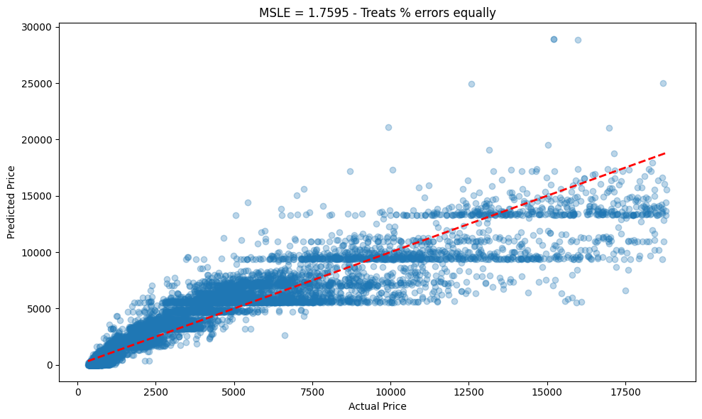
Python Code Example

import numpy as np
import seaborn as sns
from sklearn.linear_model import LinearRegression
from sklearn.metrics import mean_squared_log_error, mean_squared_error
from sklearn.model_selection import train_test_split
import matplotlib.pyplot as plt

# Load the diamonds dataset - prices span a wide range
diamonds = sns.load_dataset('diamonds')
diamonds = diamonds.dropna()
print("Price range:", diamonds['price'].min(), "to", diamonds['price'].max())

# Prepare data: Predict price based on carat
X = diamonds[['carat']].values
y = diamonds['price'].values

# Split data
X_train, X_test, y_train, y_test = train_test_split(X, y, test_size=0.2, random_state=42)

# Train model
model = LinearRegression()
model.fit(X_train, y_train)

# Predictions
y_pred = model.predict(X_test)

# Ensure no negative predictions (MSLE requires non-negative values)
y_pred = np.maximum(y_pred, 0)

# Calculate MSLE
msle = mean_squared_log_error(y_test, y_pred)
print(f"\nMean Squared Logarithmic Error (MSLE): {msle:.4f}")

# Manual calculation of MSLE
manual_msle = np.mean((np.log(y_test + 1) - np.log(y_pred + 1)) ** 2)
print(f"Manual MSLE calculation: {manual_msle:.4f}")

# Compare with MSE to see the difference
mse = mean_squared_error(y_test, y_pred)
print(f"\nFor comparison:")
print(f"MSE: {mse:.2f} (dominated by large values)")
print(f"MSLE: {msle:.4f} (treats all scales fairly)")

# Demonstrate why MSLE is useful
print("\n--- Why MSLE is useful for this data ---")
# Example 1: Small values
actual_small, pred_small = 1000, 1100  # 10% error
error_small_mse = (actual_small - pred_small)**2
error_small_msle = (np.log(actual_small + 1) - np.log(pred_small + 1))**2

# Example 2: Large values
actual_large, pred_large = 10000, 11000  # 10% error
error_large_mse = (actual_large - pred_large)**2
error_large_msle = (np.log(actual_large + 1) - np.log(pred_large + 1))**2

print(f"10% error on $1000:")
print(f"  MSE contribution: {error_small_mse:.2f}")
print(f"  MSLE contribution: {error_small_msle:.6f}")

print(f"\n10% error on $10000:")
print(f"  MSE contribution: {error_large_mse:.2f} (1000x larger!)")
print(f"  MSLE contribution: {error_large_msle:.6f} (similar!)")

# Visualize
plt.figure(figsize=(10, 6))
plt.scatter(y_test, y_pred, alpha=0.3)
plt.plot([y_test.min(), y_test.max()], [y_test.min(), y_test.max()], 'r--', lw=2)
plt.xlabel('Actual Price')
plt.ylabel('Predicted Price')
plt.title(f'MSLE = {msle:.4f} - Treats % errors equally')
plt.tight_layout()
plt.show()

Output

Price range: 326 to 18823

Mean Squared Logarithmic Error (MSLE): 1.7595
Manual MSLE calculation: 1.7595

For comparison:
MSE: 2388983.70 (dominated by large values)
MSLE: 1.7595 (treats all scales fairly)

--- Why MSLE is useful for this data ---
10% error on $1000:
  MSE contribution: 10000.00
  MSLE contribution: 0.009067

10% error on $10000:
  MSE contribution: 1000000.00 (1000x larger!)
  MSLE contribution: 0.009082 (similar!)