Mean Squared Error (MSE) / L2 Loss

Definition

MSE is the most popular and easiest to understand loss function in regression. It calculates the average of the squared differences between predicted and actual values.

Individual Loss (L2):

L (y, \hat{y}) = (y - \hat{y})^{2}

Mean Squared Error:

M S E = \frac{1}{n} \sum_{i = 1}^{n} (y_{i} - \hat{y_{i}})^{2}

Where:

$n$ = number of samples
$y_{i}$ = actual value
$\hat{y_{i}}$ = predicted value

Advantages

1. Smooth and differentiable

The MSE function ( $x^{2}$ ) is continuous and has a smooth, well-defined derivative at every point. This makes it the "gold standard" for Gradient Descent.
- Unlike Mean absolute error (MAE), which has a sharp "V" shape at zero that can cause math errors,
- MSE has a gentle "U" shape that optimization algorithms can slide down easily.
Note 👉 : Scaling features significantly improves convergence

2. Penalizes large errors heavily

Because errors are squared, a mistake of 10 units is punished 100 times more than a mistake of 1 unit.
This forces the model to prioritize fixing large mistakes. It’s ideal for scenarios where being "slightly off" is fine, but being "massively off" is a catastrophe (Medical field)

3. Efficient convergence

The gradient slowly declines as you approach the minimum, leading to stable convergence.
- The derivative of the per-sample loss is $\frac{d f}{d y} (y - \hat{y})^{2} = - 2 (y - \hat{y})$ .
- As $\hat{y}$ approaches $y$ , the gradient magnitude shrinks, leading to smaller updates near the optimum.
It matters because, as the model nears the "perfect" answer, it naturally takes smaller and smaller steps. This prevents the model from "overshooting" the target and leads to a very stable, precise final result without needing to manually tweak the learning rate as much.

4. Mathematical convenience

MSE is deeply rooted, widely used and well-understood in classical statistics.
Because it is so well-understood, it integrates perfectly with other statistical tools like ANOVA, R-squared, and Standard Deviation.

5. Unique Solutions

The MSE loss surface is strictly convex. In many linear scenarios, MSE is guaranteed to have one single "best" answer (a global minimum).

Disadvantages

1. Outlier Sensitivity (The "Panic" Effect)

Issue: Squaring the error ( $e^{2}$ ) gives disproportionate weight to large misses.
Impact: A single extreme value can dominate the loss, forcing the model to prioritize fixing one outlier at the expense of the overall "normal" data fit.

2. Interpretability & Units

Squared Units: MSE results in "units squared" (e.g., $$^{2}$ or $k g^{2}$ ). This makes the number abstract and impossible to visualize in a real-world context.
The Fix: Use RMSE if You need the loss to be in the same units as your target variable

3. The Scale & Comparison Problem

Non-Comparability: MSE is not scale-invariant. You cannot compare the MSE of a model predicting "Weight in Grams" to a model predicting "Weight in Kilograms."
Amplification: As the scales are totally different, and the squaring effect exponentially amplifies that difference massively ( $10^{2} = 100$ vs $1000^{2} = 1, 000, 000$ )

4. The Normal Distribution Assumption:

MSE is the "Maximum Likelihood Estimator" for the mean of a Normal (Gaussian) Distribution
Impact: If your errors do not follow a bell curve (for example, if they are "skewed" or have "fat tails" with many outliers)
- MSE corresponds to assuming the errors are Gaussian. If your errors are heavy-tailed or have many outliers, using MSE-based estimators is often not robust: a few extreme points can strongly influence the fit, even though the model may still be unbiased in a classical sense.
MSE squares every error, a single outlier with an error of $10$ adds $100$ to your loss, while an error of $1$ only adds $1$ . The model will "panic" over the outlier and shift its entire fit just to reduce that one large squared error, often making the predictions worse for the rest of the "normal" data points.

When to Use MSE

Your data has no or few outliers
You want to heavily penalize large errors
You're using gradient-based optimization (e.g., neural networks, linear regression)
The error distribution is approximately normal (Gaussian)

Scaling and Practical Considerations

1. Does MSE Need Scaled Data?

The short answer: Technically, No. The math of MSE works on any numbers you give it.
The real answer: Practically, Yes, your model will struggle to "see" small features if big features are shouting too loudly.

2. When does scaling helps?

★ Distance-Based Models (The "Comparison" Problem)

Models like: KNN, SVM, K-Means

These models rely on distances in the feature space, not on MSE directly. If features are on very different scales, the distance metric (e.g., Euclidean) will be dominated by large-scale features, which indirectly affects the model’s performance and the resulting MSE.
Analogy: If One feature is measured in Kilometers (1–10) and another in Millimeters (1–1,000,000), the model will think the millimeters are much more "important" just because the numbers are bigger.

★ Gradient-Based Models

Models like: Neural Networks, Linear Regression with Gradient Descent

Scaling features significantly improves convergence speed and prevents features with larger scales from dominating the loss.

★ Regularized Models

Models like: Ridge, Lasso, Elastic Net

Regularization penalizes large coefficients, so features with different scales can get unfairly treated if not standardized.
Analogy: Regularization is like a "tax" on the size of your coefficients. If your "Square Footage" is 2000 and "Bedrooms" is 3, the model naturally gives Square Footage a tiny coefficient to keep the math balanced. The "tax" will then unfairly ignore the tiny coefficient and crush the larger one. Scaling puts all features on a level playing field so the penalty is applied fairly.

3. When scaling is essential?

★ Multiple Features

If predicting house prices using both "square footage" (1000-5000) and "number of bedrooms" (1-10), the square footage will dominate MSE without scaling.
Analogy: If you predict house prices using Square Feet (2000) and Bedrooms (3), an error of 10% in square feet is 200, but 10% in bedrooms is only 0.3. When you square those ( $200^{2}$ vs ${0.3}^{2}$ ), the square footage becomes a "bully" that dominates the MSE, forcing the model to ignore the bedrooms entirely.

Before scaling: Features with larger numeric ranges contribute more to the MSE, potentially biasing the model toward optimizing those features.

After scaling: All features contribute equally to the loss based on their predictive power, not their numeric scale.

4. When scaling isn't necessary for MSE?

Tree-based models (Random Forest, XGBoost, Decision Trees): These are scale-invariant and don't benefit from normalization.
Single feature models: If you only have one predictor, scaling won't change the relative errors.

Python Code Example

import numpy as np
import pandas as pd
import seaborn as sns
import matplotlib.pyplot as plt
from sklearn.linear_model import LinearRegression
from sklearn.metrics import mean_squared_error
from sklearn.model_selection import train_test_split

# Load the tips dataset from seaborn
tips = sns.load_dataset('tips')
print("Dataset shape:", tips.shape)
print(tips.head())

# Prepare data: Predict tip based on total_bill
X = tips[['total_bill']].values
y = tips['tip'].values

# Split the data
X_train, X_test, y_train, y_test = train_test_split(X, y, test_size=0.2, random_state=42)

# Train a linear regression model
model = LinearRegression()
model.fit(X_train, y_train)

# Make predictions
y_pred = model.predict(X_test)

# Calculate MSE using sklearn
mse = mean_squared_error(y_test, y_pred)
print(f"\nMean Squared Error (MSE): {mse:.4f}")

# Manual calculation of MSE
manual_mse = np.mean((y_test - y_pred) ** 2)
print(f"Manual MSE calculation: {manual_mse:.4f}")

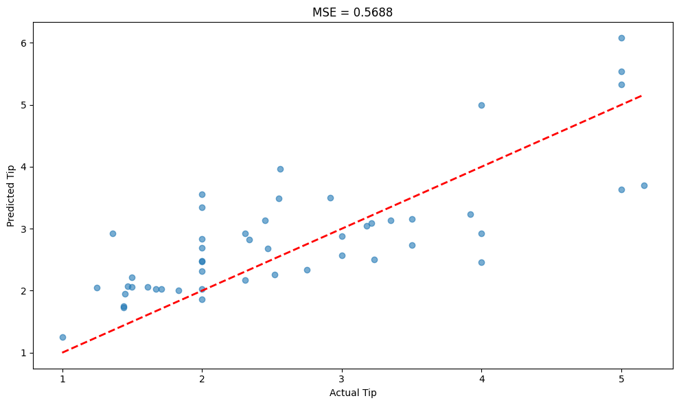
# Visualize predictions vs actual
plt.figure(figsize=(10, 6))
plt.scatter(y_test, y_pred, alpha=0.6)
plt.plot([y_test.min(), y_test.max()], [y_test.min(), y_test.max()], 'r--', lw=2)
plt.xlabel('Actual Tip')
plt.ylabel('Predicted Tip')
plt.title(f'MSE = {mse:.4f}')
plt.tight_layout()
plt.show()

Output

Dataset shape: (244, 7)
   total_bill   tip     sex smoker  day    time  size
0       16.99  1.01  Female     No  Sun  Dinner     2
1       10.34  1.66    Male     No  Sun  Dinner     3
2       21.01  3.50    Male     No  Sun  Dinner     3
3       23.68  3.31    Male     No  Sun  Dinner     2
4       24.59  3.61  Female     No  Sun  Dinner     4

Mean Squared Error (MSE): 0.5688
Manual MSE calculation: 0.5688