Mean Bias Error (MBE)
Definition
MBE calculates the average of the errors (not absolute errors), which tells us if the model has a systematic tendency to overpredict or underpredict. Unlike other metrics, it doesn't measure accuracy—it measures bias.
Individual Loss (Bias):
Mean Bias Error:
Advantages
1. Detects Systematic Bias
- Tells you if your model consistently over or underpredicts.
- Unlike accuracy metrics that focus on error magnitude, MBE reveals directional tendencies in your predictions.
2. Sign Indicates Direction
- Positive MBE = underprediction (predictions are too low)
- Negative MBE = overprediction (predictions are too high)
- The sign provides actionable insight for model correction.
3. Simple to Calculate
- No absolute values or squaring needed.
- The formula is straightforward: just the average of the raw errors.
- Computationally inexpensive and easy to explain to stakeholders.
4. Useful for Calibration
- Helps identify if you need to adjust your model's predictions systematically.
- Can directly subtract MBE from predictions to remove systematic bias.
- Essential diagnostic tool for model refinement.
Disadvantages
1. Errors Can Cancel Out
- A +10 error and a -10 error result in MBE = 0, even though the model is terrible.
- Example: A model that predicts +100 for half the data and -100 for the other half would have MBE = 0, masking the fact that it's completely wrong for every single prediction.
- This makes MBE unsuitable as a standalone accuracy measure.
2. Not a Measure of Accuracy
- MBE close to zero doesn't mean the model is good, just that it's not biased.
- A model can have perfect MBE = 0 while having enormous individual errors that happen to balance out.
- It tells you nothing about the magnitude or distribution of errors.
3. Unreliable on Its Own
- Should always be used alongside other metrics like MAE or RMSE.
- Without companion metrics, you have no idea if your predictions are actually accurate.
- MBE is a diagnostic tool, not a performance metric.
4. Can Be Misleading
- Low MBE with high individual errors is possible.
- A systematic bias in one direction might be preferable to random errors in both directions, but MBE would show the latter as "better."
- Requires careful interpretation in context with other metrics.
When to Use MBE
- You want to detect systematic bias in your model
- You need to know if predictions are consistently high or low
- You're calibrating a model and need to adjust for bias
- Used as a diagnostic tool alongside other metrics
When to Avoid MBE
- As the sole metric for model evaluation
- When you need to measure overall accuracy
- You don't care about the direction of errors
Scaling and Practical Considerations
1. Does MBE Need Scaled Data?
The short answer: Technically, No. MBE is a diagnostic metric that works on any scale.
The real answer: Practically, Yes for features (to train better models), but be careful with target scaling as it changes interpretation.
2. Key Insight: MBE Measures Bias in Original Units
- MBE tells you the average direction and magnitude of prediction errors
- Its value changes with the scale of your target variable
- Unlike percentage-based metrics, MBE is not scale-invariant
- Analogy: If you're predicting house prices, MBE = -$2,500 means you overpredict by $2,500 on average. That's immediately interpretable. But if you scale prices to 0-1, MBE = -0.025 requires mental math to understand.
3. When does scaling help?
★ Feature Scaling (Always Recommended)
Applies to all model types that benefit from scaling
- Recommended for model training (same as other metrics)
- Improves convergence for gradient-based models
- Essential for regularized models (Ridge, Lasso) to treat features fairly
- Doesn't directly affect MBE interpretation since MBE measures target bias, not feature bias
★ Target Scaling (Changes Interpretation)
Be cautious: this changes what MBE means
Without target scaling:
# MBE = -$2.50
# → Model overpredicts by $2.50 on average
# Clear, interpretable in original units ✅
With Standardization (mean=0, std=10):
# MBE = -0.25
# → Model overpredicts by 0.25 standard deviations
# Still meaningful, but requires understanding of scale ⚠️
With MinMax scaling (0-1):
# If original range is $0-$100
# MBE = -0.025
# → Model overpredicts by 0.025 in normalized units
# → That's $2.50 in original units
# Harder to interpret without reverse calculation ❌
4. Effect of Scaling on MBE
| Scenario | MBE Value | Interpretation |
|---|---|---|
| Original scale | -2.50 | Overpredict by 2.50 units ✅ Clear |
| Standardized | -0.25 | Overpredict by 0.25 std devs ✅ Statistical meaning |
| MinMax (0-1) | -0.025 | Overpredict by 2.5% of range ⚠️ Less intuitive |
5. Why Scaling Matters for MBE
- MBE is used to calibrate models (adjust predictions by subtracting MBE)
- If computed on scaled data, you must apply the correction in scaled space
- If computed on original data, you can directly adjust predictions
- Analogy: If your thermometer is consistently off by 2°C, you can just subtract 2°C from every reading. But if you're working in scaled units, you need to convert back and forth, adding complexity.
6. Best Practice for MBE
- ✅ Scale features for model training
- ✅ For reporting and interpretation: Calculate MBE on original scale
- ✅ For model calibration:
# Option 1: Calibrate on original scale (clearer) calibrated_pred = y_pred - mbe # If MBE on original scale # Option 2: Calibrate on scaled data y_pred_scaled = model.predict(X_test_scaled) mbe_scaled = np.mean(y_test_scaled - y_pred_scaled) calibrated_pred_scaled = y_pred_scaled - mbe_scaled calibrated_pred = scaler.inverse_transform(calibrated_pred_scaled) - ⚠️ If you must use scaled targets, clearly state MBE is in "standard deviation units" or "normalized units"
- MBE targets the Mean: If you minimize MBE, your model is trying to predict the Average value, but with a focus on bias, not error magnitude.
- MAE targets the Median: If you minimize MAE, your model is trying to predict the Median value.
Why this matters: MBE is about systematic error (bias), not accuracy. MAE is about error size, not direction.
Python Code Example
import numpy as np
import seaborn as sns
from sklearn.linear_model import LinearRegression
from sklearn.metrics import mean_absolute_error, mean_squared_error
from sklearn.model_selection import train_test_split
import matplotlib.pyplot as plt
# Load the mpg dataset
mpg = sns.load_dataset('mpg')
mpg = mpg.dropna()
# Prepare data
X = mpg[['horsepower', 'weight']].values
y = mpg['mpg'].values
# Split data
X_train, X_test, y_train, y_test = train_test_split(X, y, test_size=0.2, random_state=42)
# Train model
model = LinearRegression()
model.fit(X_train, y_train)
# Predictions
y_pred = model.predict(X_test)
# Calculate MBE manually (sklearn doesn't have MBE)
mbe = np.mean(y_test - y_pred)
print(f"Mean Bias Error (MBE): {mbe:.4f}")
# Interpret the result
if mbe > 0:
print(f"→ Model tends to UNDERPREDICT by an average of {abs(mbe):.2f} mpg")
elif mbe < 0:
print(f"→ Model tends to OVERPREDICT by an average of {abs(mbe):.2f} mpg")
else:
print("→ Model has no systematic bias")
# Compare with other metrics
mae = mean_absolute_error(y_test, y_pred)
rmse = np.sqrt(mean_squared_error(y_test, y_pred))
print(f"\nComparison with other metrics:")
print(f"MBE: {mbe:.4f} (shows bias direction)")
print(f"MAE: {mae:.4f} (shows average error magnitude)")
print(f"RMSE: {rmse:.4f} (penalizes large errors)")
# Demonstrate how errors cancel out
errors = y_test - y_pred
print(f"\nError statistics:")
print(f"Positive errors (underpredictions): {np.sum(errors > 0)}")
print(f"Negative errors (overpredictions): {np.sum(errors < 0)}")
print(f"MBE (net): {mbe:.4f}")
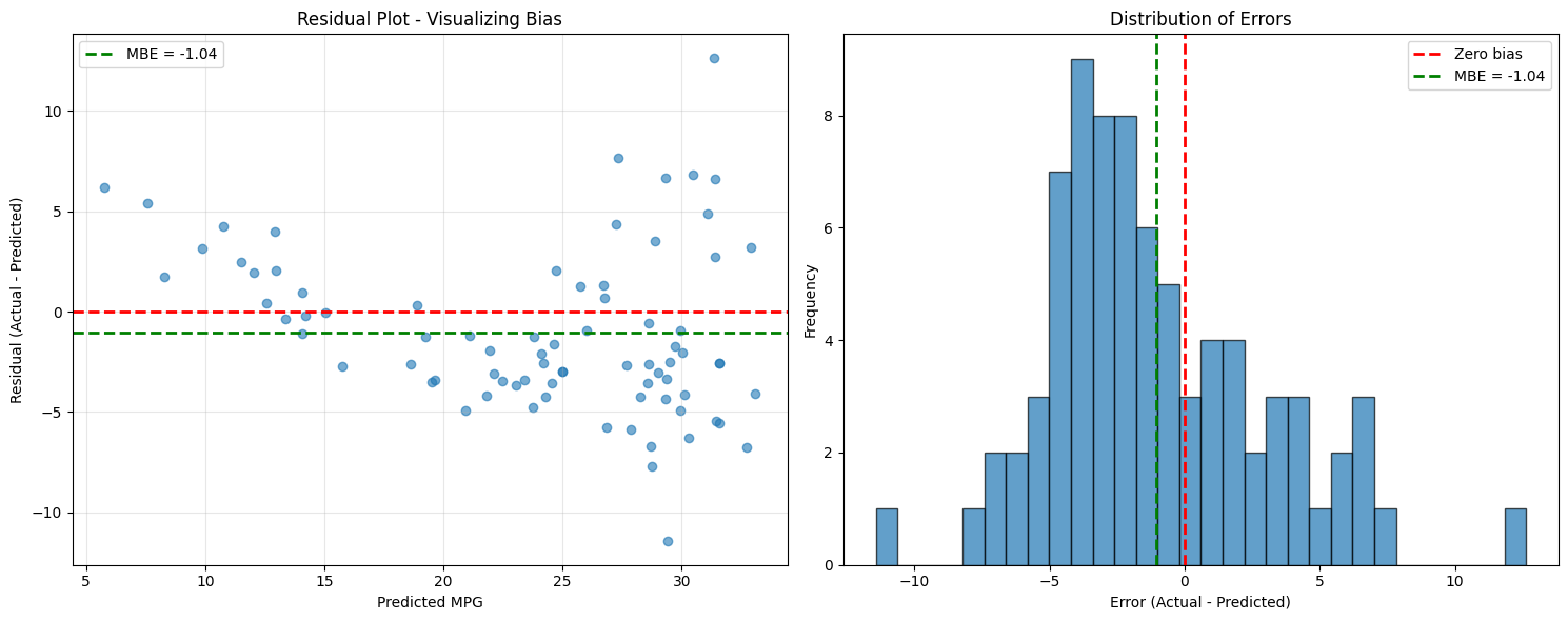
# Visualize bias
fig, axes = plt.subplots(1, 2, figsize=(15, 6))
# Plot 1: Residual plot
axes[0].scatter(y_pred, errors, alpha=0.6)
axes[0].axhline(y=0, color='r', linestyle='--', linewidth=2)
axes[0].axhline(y=mbe, color='g', linestyle='--', linewidth=2, label=f'MBE = {mbe:.2f}')
axes[0].set_xlabel('Predicted MPG')
axes[0].set_ylabel('Residual (Actual - Predicted)')
axes[0].set_title('Residual Plot - Visualizing Bias')
axes[0].legend()
axes[0].grid(True, alpha=0.3)
# Plot 2: Error distribution
axes[1].hist(errors, bins=30, alpha=0.7, edgecolor='black')
axes[1].axvline(0, color='r', linestyle='--', linewidth=2, label='Zero bias')
axes[1].axvline(mbe, color='g', linestyle='--', linewidth=2, label=f'MBE = {mbe:.2f}')
axes[1].set_xlabel('Error (Actual - Predicted)')
axes[1].set_ylabel('Frequency')
axes[1].set_title('Distribution of Errors')
axes[1].legend()
plt.tight_layout()
plt.show()
Output
Mean Bias Error (MBE): -1.0425
→ Model tends to OVERPREDICT by an average of 1.04 mpg

Comparison with other metrics:
MBE:  -1.0425 (shows bias direction)
MAE:  3.5057 (shows average error magnitude)
RMSE: 4.2180 (penalizes large errors)

Error statistics:
Positive errors (underpredictions): 26
Negative errors (overpredictions): 53
MBE (net): -1.0425