Log-Cosh Loss

Definition

Log-Cosh Loss is the logarithm of the hyperbolic cosine of the prediction error. It's a smooth approximation to the absolute error that combines advantages of both MSE and MAE. It behaves like MSE for small errors and like MAE for large errors, but it's smoother than Huber loss and doesn't require tuning a hyperparameter.

Formula:

Log-Cosh = \sum_{i = 1}^{n} \log (\cosh (\hat{y_{i}} - y_{i}))

Where $\cosh (x) = \frac{e^{x} + e^{- x}}{2}$

Advantages

1. Smooth Everywhere

Twice differentiable, providing smooth gradients for optimization.
Unlike MAE which has a sharp corner at zero, Log-Cosh maintains smoothness at all points.
This smoothness makes it ideal for gradient-based optimization methods like gradient descent.
Analogy: While MAE is like a sharp "V" where the optimizer can get confused at the bottom, Log-Cosh is like a smooth valley that guides the optimizer perfectly to the minimum.

2. Robust to Outliers

Behaves linearly for large errors, similar to MAE.
Large prediction mistakes don't dominate the loss function as they would with MSE.
For errors beyond a certain threshold, the loss grows linearly rather than quadratically.
Impact: Your model won't "panic" over outliers and sacrifice overall performance to fix one extreme value.

3. No Hyperparameter Needed

Unlike Huber loss, you don't need to tune a threshold parameter (delta).
The transition from quadratic to linear behavior happens automatically.
Reduces model complexity and eliminates one hyperparameter from cross-validation.
Why this matters: One less thing to tune means faster model development and less risk of overfitting to validation data.

4. Symmetric and Fair

Treats positive and negative errors equally.
No bias toward overprediction or underprediction.
The loss function is an even function: $\log (\cosh (x)) = \log (\cosh (- x))$ .

5. Works Well with Gradient Descent

Better convergence properties than MAE due to smoothness.
Gradients are well-behaved and never undefined.
Combines the stability of MSE near the optimum with the robustness of MAE for large errors.

Disadvantages

1. Computationally Expensive

Involves hyperbolic functions ( $\cosh$ , $\log$ ), which are slower to compute than simple operations.
Each prediction requires calculating: $e^{x} + e^{- x}$ , division by 2, and then a logarithm.
For very large datasets or real-time applications, this computational overhead can be significant.
Impact: Training time can be noticeably longer compared to MSE or MAE, especially with large neural networks.

2. Less Interpretable

The loss values don't have an intuitive meaning like MAE (average absolute error) or RMSE (root mean square error).
Difficult to explain to non-technical stakeholders: "The log of the hyperbolic cosine is 0.75" doesn't mean much.
Cannot directly translate loss value to real-world units of your target variable.
Example: MAE = 5 means "off by 5 units on average." Log-Cosh = 5 doesn't have such clear interpretation.

3. Not Always Better

May not outperform simpler loss functions (MSE, MAE) in practice.
The theoretical advantages don't always translate to better real-world performance.
Added complexity may not justify marginal improvements over Huber loss with well-tuned delta.
Reality check: If MSE or MAE already works well for your problem, Log-Cosh might be unnecessary complexity.

4. Potential for Numerical Instability

For very large errors, $\cosh (x) = \frac{e^{x} + e^{- x}}{2}$ can overflow.
When $x$ is large (e.g., $x > 100$ ), $e^{x}$ becomes astronomically large, causing numerical errors.
The Fix: Proper scaling and clipping of predictions can prevent this, but it requires awareness.
Modern implementations often include safeguards, but custom implementations need careful handling.

When to Use Log-Cosh Loss

You want smooth gradients for optimization but also robustness to outliers
You don't want to tune the hyperparameter required by Huber loss
You're using deep learning or other gradient-based methods where smoothness matters
You have some outliers but not extreme ones

When to Avoid Log-Cosh Loss

Computational efficiency is critical
You need highly interpretable metrics for reporting
Your data has extreme outliers (use Huber or MAE)
Simpler loss functions already work well for your problem

Scaling and Practical Considerations

1. Does Log-Cosh Loss Need Scaled Data?

The short answer: Technically, No. The math works on any scale.
The real answer: Practically, Yes. Scaling is highly recommended because Log-Cosh approximates different losses at different error scales.

2. Key Insight: Log-Cosh Behaves Differently at Different Error Magnitudes

The transition behavior:

Small errors (|error| < 1): Acts like MSE (quadratic) - smooth optimization
Large errors (|error| > 1): Acts like MAE (linear) - robust to outliers

Why this matters:

Without scaling, most errors might fall into the "large" category, and you essentially have MAE with extra computation
With scaling, you get balanced behavior with both smooth optimization AND outlier robustness
Analogy: Log-Cosh is like having two gears in a car. Scaling determines which gear you're using most of the time. Without scaling, you might be stuck in one gear instead of smoothly transitioning between both.

3. When does scaling help?

★ Multi-Feature Models

Always scale features to prevent large-scale features from dominating.
Features with different ranges (e.g., age: 0-100 vs income: 0-1,000,000) would cause the model to focus disproportionately on the large-range feature.
Scaling ensures all features contribute based on their predictive power, not their numeric range.

★ Neural Networks

Essential for stable gradient flow and proper weight initialization.
Unscaled features can cause vanishing or exploding gradients.
Batch normalization helps but doesn't eliminate the need for input scaling.

★ Regularized Models

Mandatory for fair regularization (Ridge, Lasso, Elastic Net).
Without scaling, regularization penalizes coefficients of small-scale features more harshly.
Analogy: Regularization is like a tax. If features aren't scaled, the "tax" unfairly punishes coefficients based on feature scale rather than importance.

★ Understanding Transition Behavior

Scaling helps you understand where Log-Cosh acts like MSE vs MAE.
With standardized features (mean=0, std=1), errors typically fall in [-3, 3] range.
This range provides balanced use of both quadratic (small errors) and linear (large errors) regions.

4. Effect of Scaling on Log-Cosh Loss

Without scaling:

# Feature range: [0, 1000]
# Errors might be: [0, 100]
# Log-Cosh treats most errors as "large" → behaves mostly like MAE
# You lose the smooth optimization benefit for small errors
# Computational cost without MSE-like benefits

With standardization:

# Features scaled to mean=0, std=1
# Errors typically in range: [-3, 3]
# Log-Cosh has balanced MSE-like (small) and MAE-like (large) regions
# Better gradient behavior across the error range
# Gets the best of both worlds

Numerical stability considerations:

# cosh(x) grows exponentially: cosh(100) = 1.3e43
# Without scaling, large errors can cause overflow in exp() calculation
# Scaling keeps errors in manageable range, typically [-5, 5]
# Prevents numerical errors and NaN values

5. Visualization of Scaling Effect

Error Range	Without Scaling	With Scaling
Small (< transition point)	Rare if features unscaled	Common - benefits from MSE-like smoothness
Large (> transition point)	Most errors here	Outliers only - benefits from MAE-like robustness
Behavior	Mostly linear (like MAE)	Balanced quadratic + linear
Optimization	Good but not optimal	Excellent gradient properties

6. Best Practice for Log-Cosh Loss

✅ Always standardize features (StandardScaler)
✅ Consider standardizing target for neural networks to keep errors in [-3, 3] range

✅ Monitor actual error magnitudes to ensure balanced behavior:

# Check error distribution
errors = y_test - y_pred
print(f"Error std: {np.std(errors):.2f}")
print(f"Errors in [-1, 1]: {np.mean(np.abs(errors) < 1) * 100:.1f}%")
print(f"Errors > 2: {np.mean(np.abs(errors) > 2) * 100:.1f}%")

⚠️ If most errors are > 3 even after scaling, consider using MAE directly
⚠️ If most errors are < 0.1 after scaling, consider using MSE directly

⚠️ Add error clipping for extreme cases to prevent numerical overflow:

# Clip predictions to prevent extreme errors
y_pred_clipped = np.clip(y_pred, y_train.min() - 3*y_train.std(), 
                                  y_train.max() + 3*y_train.std())

7. Comparison with Huber Loss

Huber Loss: You set delta (threshold) explicitly → need to adjust delta if you change scaling
Log-Cosh Loss: Transition is automatic around |error| ≈ 1 → scaling determines what counts as "1"
Both benefit from standardization, but Log-Cosh is less sensitive to scale choice
Trade-off: Huber gives more control, Log-Cosh requires less tuning

Python Code Example

import numpy as np
import seaborn as sns
from sklearn.linear_model import LinearRegression
from sklearn.metrics import mean_absolute_error, mean_squared_error
from sklearn.model_selection import train_test_split
import matplotlib.pyplot as plt

# Define Log-Cosh Loss function
def log_cosh_loss(y_true, y_pred):
    """
    Logarithm of the hyperbolic cosine of the prediction error.
    """
    error = y_pred - y_true
    return np.mean(np.log(np.cosh(error)))

# Load the tips dataset
tips = sns.load_dataset('tips')

# Add some outliers
X = tips[['total_bill']].values
y = tips['tip'].values
y_with_outliers = y.copy()
y_with_outliers[[5, 10, 15, 20]] = [25, 30, 28, 35]  # Add outliers

# Split data
X_train, X_test, y_train, y_test = train_test_split(X, y_with_outliers, test_size=0.2, random_state=42)

# Train model
model = LinearRegression()
model.fit(X_train, y_train)

# Predictions
y_pred = model.predict(X_test)

# Calculate Log-Cosh Loss
log_cosh = log_cosh_loss(y_test, y_pred)
print(f"Log-Cosh Loss: {log_cosh:.4f}")

# Compare with other loss functions
mse = mean_squared_error(y_test, y_pred)
mae = mean_absolute_error(y_test, y_pred)
rmse = np.sqrt(mse)

print(f"\nComparison of loss functions:")
print(f"MSE:       {mse:.4f} (very sensitive to outliers)")
print(f"RMSE:      {rmse:.4f} (sensitive to outliers)")
print(f"MAE:       {mae:.4f} (robust to outliers)")
print(f"Log-Cosh:  {log_cosh:.4f} (balanced approach)")

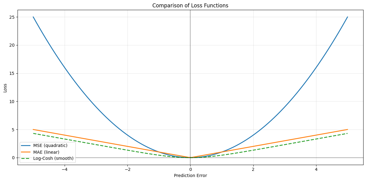
# Visualize how different loss functions behave
errors = np.linspace(-5, 5, 100)

# Calculate loss for each error magnitude
mse_loss = errors ** 2
mae_loss = np.abs(errors)
log_cosh_loss_curve = np.log(np.cosh(errors))

# Plot
plt.figure(figsize=(12, 6))
plt.plot(errors, mse_loss, label='MSE (quadratic)', linewidth=2)
plt.plot(errors, mae_loss, label='MAE (linear)', linewidth=2)
plt.plot(errors, log_cosh_loss_curve, label='Log-Cosh (smooth)', linewidth=2, linestyle='--')
plt.xlabel('Prediction Error')
plt.ylabel('Loss')
plt.title('Comparison of Loss Functions')
plt.legend()
plt.grid(True, alpha=0.3)
plt.axhline(y=0, color='k', linestyle='-', alpha=0.3)
plt.axvline(x=0, color='k', linestyle='-', alpha=0.3)
plt.tight_layout()
plt.show()

Output

Log-Cosh Loss: 1.3404

Comparison of loss functions:
MSE:       28.6915 (very sensitive to outliers)
RMSE:      5.3564 (sensitive to outliers)
MAE:       1.7742 (robust to outliers)
Log-Cosh:  1.3404 (balanced approach)