Square Root, Square, and Reciprocal Transformations

★ Square Root Transformation (√x)

---
config:
  theme: 'base'
  layout: 'tidy-tree'
  fontSize: 5
  font-family: '"Gill Sans", sans-serif'
---
mindmap
    root(Square root √x)
	    ❌ Avoid When
		    Negative values present
		    Already normal data 
		    Left-skewed data
		    Need stronger correction
	    ✅ Use When
		    Right-skewed data
		    Count data Poisson
		    Moderate skewness
		    Stabilize variance

I. The Mechanics

Formula:

X_{transformed} = \sqrt{X}

What it does: The square root transformation compresses larger values more than smaller ones, pulling the "long tail" on the right toward the center. It's a moderate transformation—stronger than standardization but gentler than logarithmic transformation.

II. When Square Root Transformation Shines

1. Count Data and Poisson Distributions

When dealing with frequencies, event counts, or any data following a Poisson distribution:

Website clicks, page views
Number of accidents or incidents
Customer visits, transaction counts
Word frequencies in text data

Why it works: Count data naturally exhibits variance that increases with the mean (heteroscedasticity). Square root transformation stabilizes this variance.

2. Moderate Right Skewness

When your data is right-skewed but not extremely so:

Income distributions (when not too extreme)
Age distributions in specific populations
Response times, reaction times
Physical measurements (height, weight in certain contexts)

3. Converting Non-Linear to Linear Relationships

When scatter plots show a curved relationship that could be linearized for regression models.

4. Stabilizing Variance (Heteroscedasticity)

When your residuals fan out as predictions increase, square root transformation often stabilizes variance without over-correcting.

III. When to Choose Something Else

1. Negative Values Present

Square root of negative numbers is undefined (in real numbers).

Better alternative: PowerTransformer (Yeo-Johnson) handles negative values automatically without manual adjustments.

2. Already Normal or Near-Normal Data

If your distribution is already symmetric, square root transformation will introduce left skew.

Better approach: Stick with StandardScaler or leave data as-is.

3. Features with Left Skew

Square root transformation will make left skewness worse.

Better alternative: Use Square Transformation to correct left skew.

4. Extreme Right Skewness

When your skew is severe (exponential growth patterns), square root may be too gentle.

Better alternatives: Log Transformation or #Reciprocal Transformation (1/x) provide stronger compression.

IV. Advantages

Moderate compression: Doesn't over-correct like log transformation
Variance stabilization: Particularly effective for count data
Preserves zero: √0 = 0, maintaining meaningful zero values
Interpretable: Still relatively intuitive (taking the square root)
Computationally efficient: Simple mathematical operation

V. Limitations

Requires non-negative values: Cannot handle negative numbers
Partial correction: May not fully normalize heavily skewed data
Can create left skew: If applied to already-normal or left-skewed data

★ Square Transformation (x²)

---
config:
  theme: 'base'
  layout: 'tidy-tree'
  fontSize: 5
  font-family: '"Gill Sans", sans-serif'
---
mindmap
    root(Square x²)
	    ❌ Avoid When
		    Right-skewed data
		    Very large value ranges
		    Risk of overflow
		    Computational constraints
	    ✅ Use When
		    Left-skewed data
		    Values clustered high
		    Test scores distributions
		    Need to amplify differences

I. The Mechanics

Formula:

X_{transformed} = X^{2}

What it does: The square transformation does the opposite of square root—it amplifies differences by magnifying larger values disproportionately more than smaller ones.

II. When Square Transformation Shines

1. Left-Skewed Distributions

When most of your data clusters at the high end with a long tail toward zero:

Test scores where most students performed well
Survey responses clustered at high ratings
Quality metrics with ceiling effects
Completion rates or success percentages

2. Amplifying Important Differences

When you want to emphasize distinctions at the upper range:

Prioritizing high-value customers
Emphasizing top performers
Reward functions in reinforcement learning

3. Creating Polynomial Features

In feature engineering for linear models, squaring creates interaction effects and captures non-linear relationships.

III. When to Choose Something Else

1. Right-Skewed Data

Squaring will dramatically worsen right skewness, pushing outliers even further out.

Better alternatives: Use Square Root Transformation, Log Transformation, or Reciprocal Transformation.

2. Very Large Value Ranges

Squaring large numbers can lead to computational overflow or create extreme outliers that dominate your model.

Better approach: Apply StandardScaler or MinMaxScaler first, then square, or use QuantileTransformer.

3. Need to Maintain Interpretability

Squared values lose intuitive meaning—squared income or squared age is hard to explain to stakeholders.
Better approach: Use RobustScaler or document transformations thoroughly.

VI. Advantages

Corrects left skew: Effective for distributions clustered at high values
Amplifies differences: Emphasizes distinctions at upper ranges
Handles all real numbers: Works with positive and negative values
Simple to implement: Basic mathematical operation

V. Limitations

Worsens right skew: Catastrophic if applied to wrong distribution
Risk of overflow: Large values can become computationally problematic
Interpretation difficulty: Squared units lose intuitive meaning
Sensitive to outliers: Magnifies extreme values even more

★ Reciprocal Transformation (1/x)

---
config:
  theme: 'base'
  layout: 'tidy-tree'
  fontSize: 5
  font-family: '"Gill Sans", sans-serif'
---
mindmap
    root(Reciprocal 1/x)
	    ❌ Avoid When
		    Contains zeros
		    Need preserved order
		    Moderate skewness
		    Interpretability matters
	    ✅ Use When
		    Extreme right skew
		    Rates and ratios
		    Inverse relationships
		    Time-to-event data

I. The Mechanics

Formula:

X_{transformed} = \frac{1}{X}

What it does: The reciprocal transformation completely inverts your data's scale—large values become tiny, small values become large. It's the strongest transformation for extreme right skewness.

II. When Reciprocal Transformation Shines

1. Extreme Right Skewness

When your data has exponential growth patterns that even log transformation struggles with:

Response times with extreme outliers
Failure rates or error frequencies
Survival analysis data

2. Rates and Ratios with Physical Meaning

When the inverse has a natural interpretation:

Converting "miles per gallon" to "gallons per mile"
Converting "items per hour" to "hours per item"
Speed to time relationships

3. Time-to-Event Data

When smaller values (faster events) should have more weight:

Processing times
Turnaround times
Service completion times

4. Inverse Relationships

When the relationship between variables is fundamentally inverse:

Distance and gravitational force
Price and demand (in some contexts)

III. When to Choose Something Else

1. Contains Zeros

Division by zero is undefined—this is a deal-breaker.

Better alternatives: Add a small constant (1/x+c) or use Log Transformation (handles zeros better with log1p).

2. Need to Preserve Order

Reciprocal reverses ranking—largest becomes smallest. While you can use -1/x to preserve order, this adds complexity.

Better alternative: Log Transformation maintains order while compressing range.

3. Moderate Skewness

Reciprocal is often overkill for mild to moderate skewness.

Better alternatives: Try Square Root or Log Transformation first—they're gentler and more interpretable.

4. Interpretability Matters

Reciprocal values are often unintuitive to explain to non-technical stakeholders.

Better approach: Use PowerTransformer with well-documented parameters, or stick with more interpretable transformations.

Advantages

Strongest compression: Most effective for extreme right skewness
Meaningful inverses: Natural interpretation for rates and ratios
Handles large ranges: Can bring massive scales to manageable sizes
Mathematical properties: Useful in specific modeling contexts

Limitations

Cannot handle zeros: Fatal flaw for many datasets
Reverses order: Requires negation to maintain ranking
Over-correction risk: Can create left skew if data isn't extremely skewed
Interpretation complexity: Reciprocal units are often confusing

Practical Implementation

import numpy as np
import pandas as pd
import matplotlib.pyplot as plt
import seaborn as sns
from scipy import stats

# Generate different types of skewed data
np.random.seed(42)

# Right-skewed data (for square root)
right_skewed = np.random.exponential(scale=50, size=1000)

# Left-skewed data (for square)
left_skewed = 100 - np.random.exponential(scale=20, size=1000)

# Extreme right-skewed data (for reciprocal)
extreme_right = np.random.pareto(a=1.5, size=1000) * 10 + 1

# Apply transformations
sqrt_transformed = np.sqrt(right_skewed)
square_transformed = left_skewed ** 2
reciprocal_transformed = 1 / extreme_right

# Visualization
fig, axes = plt.subplots(3, 4, figsize=(20, 12))

# Square Root Transformation
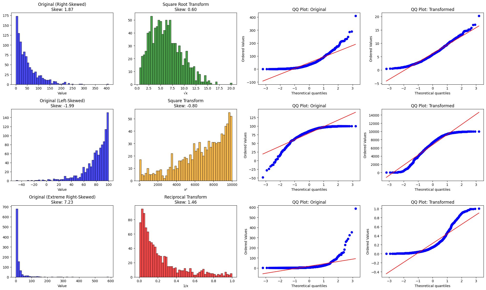
axes[0, 0].hist(right_skewed, bins=50, alpha=0.7, color='blue', edgecolor='black')
axes[0, 0].set_title(f'Original (Right-Skewed)\nSkew: {stats.skew(right_skewed):.2f}')
axes[0, 0].set_xlabel('Value')

axes[0, 1].hist(sqrt_transformed, bins=50, alpha=0.7, color='green', edgecolor='black')
axes[0, 1].set_title(f'Square Root Transform\nSkew: {stats.skew(sqrt_transformed):.2f}')
axes[0, 1].set_xlabel('√x')

stats.probplot(right_skewed, dist='norm', plot=axes[0, 2])
axes[0, 2].set_title('QQ Plot: Original')

stats.probplot(sqrt_transformed, dist='norm', plot=axes[0, 3])
axes[0, 3].set_title('QQ Plot: Transformed')

# Square Transformation
axes[1, 0].hist(left_skewed, bins=50, alpha=0.7, color='blue', edgecolor='black')
axes[1, 0].set_title(f'Original (Left-Skewed)\nSkew: {stats.skew(left_skewed):.2f}')
axes[1, 0].set_xlabel('Value')

axes[1, 1].hist(square_transformed, bins=50, alpha=0.7, color='orange', edgecolor='black')
axes[1, 1].set_title(f'Square Transform\nSkew: {stats.skew(square_transformed):.2f}')
axes[1, 1].set_xlabel('x²')

stats.probplot(left_skewed, dist='norm', plot=axes[1, 2])
axes[1, 2].set_title('QQ Plot: Original')

stats.probplot(square_transformed, dist='norm', plot=axes[1, 3])
axes[1, 3].set_title('QQ Plot: Transformed')

# Reciprocal Transformation
axes[2, 0].hist(extreme_right, bins=50, alpha=0.7, color='blue', edgecolor='black')
axes[2, 0].set_title(f'Original (Extreme Right-Skewed)\nSkew: {stats.skew(extreme_right):.2f}')
axes[2, 0].set_xlabel('Value')

axes[2, 1].hist(reciprocal_transformed, bins=50, alpha=0.7, color='red', edgecolor='black')
axes[2, 1].set_title(f'Reciprocal Transform\nSkew: {stats.skew(reciprocal_transformed):.2f}')
axes[2, 1].set_xlabel('1/x')

stats.probplot(extreme_right, dist='norm', plot=axes[2, 2])
axes[2, 2].set_title('QQ Plot: Original')

stats.probplot(reciprocal_transformed, dist='norm', plot=axes[2, 3])
axes[2, 3].set_title('QQ Plot: Transformed')

plt.tight_layout()
plt.show()

# Print statistics
print("Square Root Transformation:")
print(f"  Original Skew: {stats.skew(right_skewed):.3f}")
print(f"  Transformed Skew: {stats.skew(sqrt_transformed):.3f}\n")

print("Square Transformation:")
print(f"  Original Skew: {stats.skew(left_skewed):.3f}")
print(f"  Transformed Skew: {stats.skew(square_transformed):.3f}\n")

print("Reciprocal Transformation:")
print(f"  Original Skew: {stats.skew(extreme_right):.3f}")
print(f"  Transformed Skew: {stats.skew(reciprocal_transformed):.3f}")

The Bottom Line

These three transformations are surgical tools in your feature engineering toolkit, each designed for specific distributional challenges:

Square Root (√x): Your go-to for moderate right skewness, especially count data. It's the Goldilocks transformation—not too strong, not too weak.
Square (x²): The specialist for left-skewed data. Use it when values cluster at the high end, but be cautious with large ranges.
Reciprocal (1/x): The heavy artillery for extreme right skewness. Powerful but requires careful handling (watch for zeros and reversed order).

However, in modern machine learning workflows, you might not need to choose manually. PowerTransformer with Box-Cox (for positive data) or Yeo-Johnson (for any data) can automatically find the optimal power transformation. Consider these manual transformations when:

You understand your data's specific distribution
The transformation has physical or domain meaning
You need explainability (manual transformations are easier to document)
PowerTransformer over-fits or produces unexpected results

Before applying any transformation, always visualize your data first. A histogram and QQ plot will tell you immediately which transformation (if any) makes sense. And remember: not all skewed data needs transformation—tree-based models work perfectly fine with skewed distributions.

The best transformation is the one that serves your model's needs while preserving interpretability.