Power Transformer

A Power Transformer is a data preprocessing tool that uses mathematical power functions to transform data from any distribution—especially skewed or bimodal distributions—into a Gaussian (Normal) distribution. This process stabilizes the variance of the features and makes the data more "digestible" for machine learning models that assume normality.

---
config:
  theme: 'base'
  layout: 'tidy-tree'
  fontSize: 5
  font-family: '"Gill Sans", sans-serif'
---
mindmap
	root(PowerTransformer)
		Do Not Use When
			TreeBased Models
			Sparse Data
			Mild Skewness
			Sensitive to Outliers
			Strict Range requirements
		Use when
			Heavily Skewed
			Bimodal
			Need Gaussian distribution
		Strategies
			Yeo-Johnson 
			Box-Cox

I. Features

• Normalizes Skewed or Bimodal Data: Transforms data from any distribution—especially skewed or bimodal—towards a Gaussian (Normal) distribution.
• Variance Stabilization: Addresses heteroscedasticity (when the spread/variance of data changes with the value of the variable) by making variance more consistent across the range.
• Automatic Lambda Optimization: Determined by finding the optimal value of a parameter, called the lambda ($\lambda$)
• Standardization: By default, scales output to have mean 0 and standard deviation 1.
• Strategies for Power Transformer
  • Yeo-Johnson method works for positive, zero, and negative values;
  • Box-Cox requires strictly positive data.

II. Best Use Case

• Linear Models: Improves performance of models that assume normality (e.g., Linear Regression, Logistic Regression, LDA).
• Heteroscedastic Data: When variance increases with feature values, power transformation helps stabilize it.
• Bimodal or Heavily Skewed Data: Useful for pulling apart or compressing distributions to be more normal-like.
• Preprocessing for Statistical Tests: When statistical tests require normality of features.

III. When NOT to Use It

• Tree-Based Models: Random Forests, XGBoost, and Decision Trees do not require normally distributed features; transformation adds unnecessary complexity.
• Sparse Data: Power transformation destroys sparsity (turns zeros into non-zeros); use MaxAbsScaler for sparse data.
• Strict Range Requirements: If your model or downstream process requires features in a specific range (e.g., 0–1 for image processing), use MinMaxScalar.
• Mild Skewness: For mild skewness, simpler transformations (like log or square root) may suffice and be more interpretable.

IV. Pros

• Improves Model Performance: Especially for algorithms sensitive to feature distribution.
• Handles All Data Types: Yeo-Johnson works with negative, zero, and positive values.
• Reduces Heteroscedasticity: Makes variance more uniform, improving statistical validity.

V. Cons

• Computationally Intensive: Needs to optimize ($\lambda$) for each feature, making it slower than standard scaling.
• Reduced Interpretability: Transformed values are harder to explain to non-technical stakeholders.
• Sensitive to Outliers: Extreme values can distort the transformation and the optimal ($\lambda$).
• Destroys Sparsity: Not suitable for sparse datasets.

VI. Code Snippet

★ Box-Cox Transformation

from scipy.stats import boxcox

# Only for positive values
df['boxcox_feature'], lambda_param = boxcox(df['feature'])

★ Yeo-Johnson Transformation

from sklearn.preprocessing import PowerTransformer

# Handles negative values
pt = PowerTransformer(method='yeo-johnson')
df['yeo_johnson_feature'] = pt.fit_transform(df[['feature']])

Practical Implementation

import pandas as pd
import numpy as np
import matplotlib.pyplot as plt
import seaborn as sns
import scipy.stats as stats

# Loading Dataset
from sklearn.datasets import fetch_california_housing
housing = fetch_california_housing()

# Convert to Dataframe and target
X = pd.DataFrame(housing.data, columns=housing.feature_names)
y = housing.target

data = np.array(X['Population'])

# Applying Power Transformation
pt = PowerTransformer(method='yeo-johnson', standardize=True)
log_data = pt.fit_transform(data.reshape(-1,1))

# flatten log_data for plotting, and set titles on correct axes
log_data_flat = np.array(log_data).flatten()

# Create subplots
fig, axes = plt.subplots(1, 4, figsize=(18, 4))

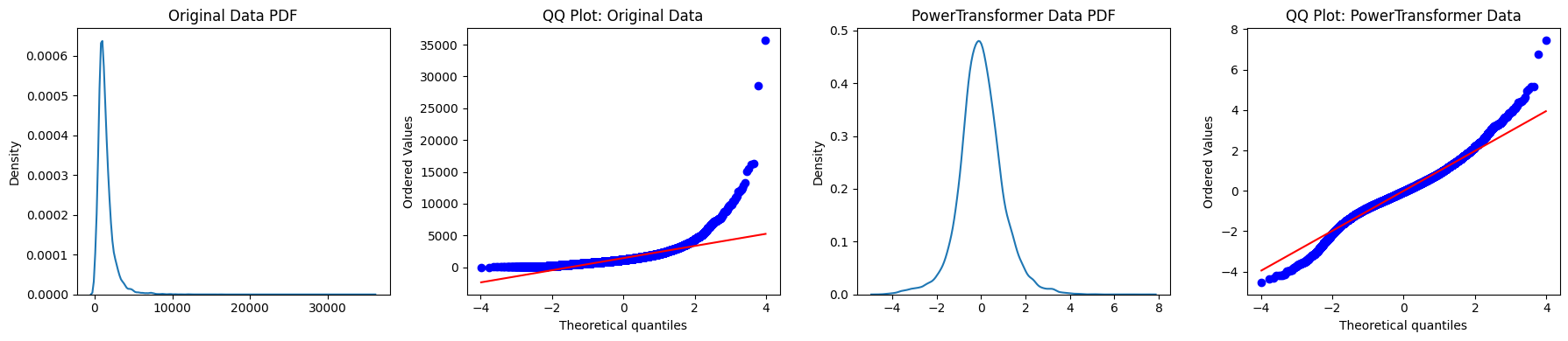
# Original Data KDE Plot
sns.kdeplot(data, ax=axes[0])
axes[0].set_title('Original Data PDF')

# Original Data QQ Plot
stats.probplot(data, dist='norm', plot=axes[1])
axes[1].set_title('QQ Plot: Original Data')

# PowerTransformed Data KDE Plot
sns.kdeplot(log_data_flat, ax=axes[2])
axes[2].set_title('PowerTransformed Data PDF')

# Power-Transformed Data QQ Plot
stats.probplot(log_data_flat, dist='norm', plot=axes[3])
axes[3].set_title('QQ Plot: PowerTransformed Data')

# Adjust layout and display
plt.tight_layout()
plt.show()