I. What is Polynomial Transformation?
The Big Picture
Imagine you're trying to predict house prices using only square footage. You fit a simple linear model and get a straight line. But what if the relationship isn't straight? What if bigger houses don't just add value linearly—maybe they add value exponentially because luxury buyers pay premium prices for space?
This is where polynomial transformation comes in. It's a feature engineering technique that helps us model non-linear relationships by creating new features that are powers or cross-products of our original features.
💭 Simple analogy: Think of it as "bending" your straight line (linear regression) so it can fit a curved set of data points. Instead of forcing a straight ruler onto a curved surface, you're making the ruler flexible.
The Math Behind It
A polynomial transformation creates new features by raising existing numeric features to powers and (optionally) creating interaction terms.
Example 1: Single feature
If you have one feature
So if square footage = 1000, you now have:
- Original: 1000
- Squared: 1,000,000
Example 2: Two features
If you have two features,
That
II. When Should You Use Polynomial Transformation?
Here's the golden rule: Use polynomial features when you have a non-linear relationship but want to keep using a linear model.
1. It Depends on Your Model
Not all models benefit from polynomial features. Let's break this down:
✅ Models that LOVE polynomial features:
These are models that assume linearity in their inputs:
- Linear Regression / Ridge / Lasso / Elastic Net
- Logistic Regression
- Linear SVM
- Generalized Linear Models (GLMs)
Why? Because these models can only draw straight lines (or flat planes in higher dimensions). By giving them
❌ Models that DON'T need polynomial features:
- Tree-based models (Random Forest, XGBoost, Decision Trees)
- Neural Networks
Why? These models can already capture non-linearities directly. Trees split on different thresholds, and neural networks use activation functions. Adding polynomial features to these models is usually redundant and just makes training slower.
When to still use polynomial features despite having complex models:
You might still use them if you need a model that's interpretable. For example, saying "sales increase with the square of advertising spend" is much easier to explain to a business stakeholder than "the neural network found a pattern."
2. You're Seeing Signs of Underfitting
An underfit model shows high error on both training and test data. It's like trying to fit a straight line through data that clearly curves.
Look at this example—we're trying to approximate part of a cosine function:
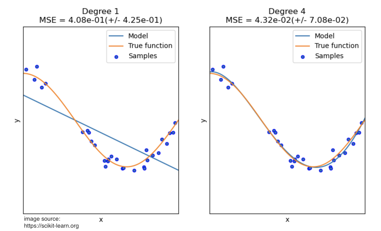
Notice how:
- The linear model (degree 1) completely misses the curve—classic underfitting
- The degree 4 polynomial captures the true pattern almost perfectly
- The degree 4 model fits the training points well without chasing every tiny fluctuation (which would be overfitting)
Red flags for underfitting:
- Your training error is high
- Your model is "too simple" for the complexity of the data
- Your residual plots show systematic patterns (not random scatter)
III. How to Select Features for Transformation?
You shouldn't blindly apply polynomial features to every variable. It adds complexity and can hurt performance. Here’s a practical guide to choosing the right features to transform.
1. Visual Inspection: Scatter Plots
This is the most direct method. For each numeric feature, create a scatter plot of that feature against your target variable.
- What to plot: Feature on the x-axis, Target on the y-axis.
- What to look for: Add a LOESS smoothing line (Locally Estimated Scatterplot Smoothing) to your plot. This line helps reveal the underlying trend without making any assumptions about the relationship.
- If the LOESS line is mostly straight, the relationship is linear. Leave the feature as is.
- If the LOESS line shows a clear curve (like a U-shape, an inverted U, or an S-curve), that feature is a prime candidate for a polynomial transformation.
!500
In this example, the LOESS line (in red) clearly shows a curve, suggesting a polynomial term would be beneficial.
2. Model Diagnostics: Residual Plots
If you've already built a linear model, its mistakes can tell you what it's missing. A residual is the error of a prediction (Actual Value - Predicted Value).
- What to plot: Your model's predictions (or a feature) on the x-axis and the residuals on the y-axis.
- What to look for:
- Random, shapeless cloud of points around zero: This is good! It means your model is capturing the underlying pattern and the errors are just random noise. No transformation needed.
- A clear pattern or curve (like a U-shape): This is a red flag! It means your linear model is systematically failing to capture a non-linear relationship. The feature causing this pattern needs a polynomial term.
!500
A curved pattern in the residuals is a classic sign that you need to account for non-linearity.
3. Domain Knowledge
Sometimes, you know a relationship should be non-linear based on real-world principles. Don't ignore this!
- Physics: The kinetic energy of an object is
. If you're predicting energy from velocity, you know a term is required. - Economics: The principle of diminishing returns suggests that the benefit of adding more of something (like advertising spend) eventually levels off. This often follows a quadratic (
) or logarithmic pattern. - Biology: The dose-response relationship in medicine is often non-linear.
4. Interaction Terms
Don't forget that polynomial features can also model how two features work together. If you suspect the effect of one feature depends on the level of another, you should include an interaction term (
- Example: In real estate, the value of having an extra bedroom (
bedrooms) is much higher if the house is large (sqft). The interaction termbedrooms * sqftwould capture this combined effect.
IV. What Power (Degree) Should You Use?
Choosing the degree is a balancing act. Too low, and you underfit. Too high, and you overfit. Here’s a guide to getting it right.
The Rule of Thumb: Keep it Simple
In 90% of real-world machine learning, you should stay between Degree 2 and Degree 3.
-
Degree 2 (
): This is your workhorse. It captures simple, common non-linear patterns like parabolas. Use it for: - Diminishing returns: The effect of a feature weakens as its value increases.
- Accelerating growth: The effect of a feature strengthens as its value increases.
-
Degree 3 (
): This is for more complex curves. Use it when your data shows an "S-curve" shape, where the effect starts slow, accelerates, and then flattens out. -
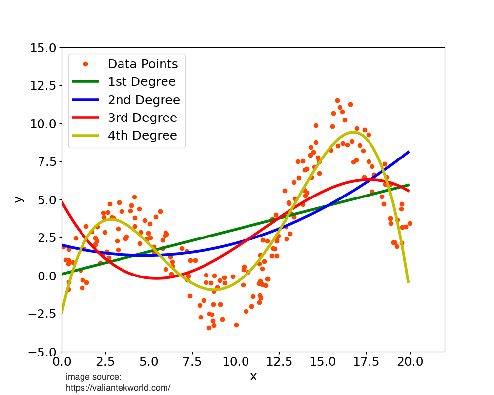
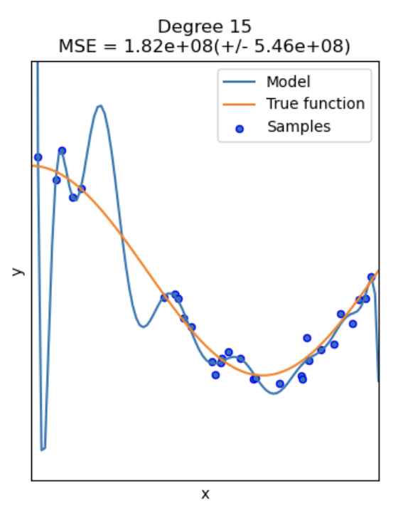
Degree 4+: Dangerous Territory. Avoid higher degrees unless you have a very strong theoretical reason (e.g., from physics).
- Why? Higher-degree polynomials can create wild, complex curves that fit your training data perfectly but fail spectacularly on new, unseen data. This is overfitting. The model learns the noise, not the signal.
The high-degree polynomial (green line) wiggles to catch every data point, making it a poor general model.
How to Find the Best Degree: A Practical Approach
You can't always "see" the best degree, especially with many features. Use a methodical, data-driven approach.
- Start with Degree 1 (Linear): Fit a simple linear model and establish a baseline performance metric (like R-squared for regression).
- Try Degree 2: Create degree-2 polynomial features and retrain your model.
- Did the performance on your validation set improve significantly? If yes, this is a good sign.
- Cautiously Try Degree 3: If degree 2 gave a good boost, try degree 3.
- If performance improves again, great.
- If it improves only slightly, or if your validation performance gets worse, then stick with Degree 2. The added complexity isn't worth it.
If you must use a higher degree (e.g., 3 or 4), you must pair it with a regularized model like Ridge or Lasso Regression.
- How it helps: Regularization adds a penalty for large coefficients. It automatically "shrinks" the coefficients of the less useful polynomial terms towards zero, effectively performing automated feature selection and reducing the risk of overfitting.
V. The Importance of Scaling
When you create polynomial features, especially with degrees higher than 1, the new features can have vastly different scales from each other. For example, if a feature x ranges from 1 to 100, x^2 will range from 1 to 10,000. This huge difference in scale can cause serious problems for many machine learning models.
Scaling your data is not just recommended; it's often required for the model to perform correctly.
Which Models Are Sensitive to Scale?
- Models with Regularization (Ridge, Lasso, Elastic Net): Scaling is mandatory. Regularization works by penalizing the size of coefficients. If features have different scales, the penalty will be applied unfairly. A feature with a large scale (like our
x^2example) will have a naturally smaller coefficient, and the model might mistakenly think it's less important. - Distance-Based Models (SVM, KNN): Scaling is mandatory. These models depend on calculating distances between data points. Features with larger scales will dominate these calculations, and the model will effectively ignore the contributions of features with smaller scales.
- Gradient-Based Models (Linear/Logistic Regression, Neural Networks): Scaling is highly recommended. It helps the optimization algorithm (like gradient descent) converge much faster and more smoothly. Unscaled features can create a difficult, elongated error surface that is slow to navigate.
The Correct Order of Operations: Scale THEN Transform
The best practice is to standardize your features before applying the polynomial transformation.
Workflow:
StandardScaler→PolynomialFeatures→Model
Here’s why this is the preferred method:
- Prevents Numerical Instability: If you create polynomial features first from unscaled data, you can end up with extremely large numbers (e.g., 1000^3 = 1,000,000,000). This can cause numerical overflow errors during model training. Scaling first keeps all values in a controlled range (e.g., around -3 to 3 for
StandardScaler). - Reduces Multicollinearity: Centering the data by scaling (subtracting the mean) before creating polynomial terms helps reduce the correlation between a feature and its powers (e.g., between
and ). This makes the model's coefficients more stable and interpretable.
While you can scale after creating polynomial features, it's less ideal because you miss out on the benefits above.
If your model uses regularization, distances, or gradients, and you are creating polynomial features, you must scale your data. The best way to do this is to scale first, then apply the polynomial transformation.
VI. Risks and Disadvantages
While powerful, polynomial features are not a free lunch. You must be aware of the risks involved.
1. Overfitting
This is the biggest danger. As you increase the polynomial degree, the model becomes more flexible and can create very complex curves. A high-degree polynomial will fit your training data almost perfectly, but it will have learned the noise in your data, not the underlying signal. When you show it new data, its predictions will be wild and unreliable.
Mitigation:
- Stick to low degrees (2 or 3).
- Use a validation set to check if performance on unseen data is actually improving.
- Use regularization (Ridge or Lasso) to penalize complexity.
2. Feature Explosion
The number of new features grows exponentially with the degree and the number of original features.
- Formula: For
poriginal features and degreed, the number of new features is. - Example:
- 5 features, degree 2 → 20 new features.
- 10 features, degree 3 → 285 new features.
- 20 features, degree 4 → 10,625 new features!
This leads to a very high-dimensional dataset, which can make training slow and memory-intensive (the "Curse of Dimensionality").
Mitigation:
- Apply polynomial features only to a small, selected subset of features that you know have a non-linear relationship with the target.
- Avoid using high degrees.
3. Multicollinearity
A feature and its powers (e.g.,
Mitigation:
- Scale your data first! Centering the data by using
StandardScalersignificantly reduces the correlation between linear and quadratic terms. - Use a regularized model like Ridge Regression, which is specifically designed to handle multicollinearity better than standard linear regression.
VII. Python Implementation with Scikit-Learn
The best way to implement polynomial regression is by using a Pipeline. This ensures that your steps (scaling, transformation) are applied correctly and prevents data leakage from your test set.
Here is a complete, commented example.
import numpy as np
import matplotlib.pyplot as plt
from sklearn.model_selection import train_test_split
from sklearn.linear_model import LinearRegression
from sklearn.preprocessing import PolynomialFeatures, StandardScaler
from sklearn.pipeline import Pipeline

# 1. Create some sample non-linear data
np.random.seed(42)
X = np.sort(5 * np.random.rand(80, 1), axis=0)
y = np.sin(X).ravel() + np.random.randn(80) * 0.1

# 2. Split data into training and testing sets
X_train, X_test, y_train, y_test = train_test_split(X, y, test_size=0.2, random_state=42)

# 3. Create a pipeline
# This is the key! It chains together the steps of our modeling process.
# We will compare a simple linear model to a polynomial one.

# Define the degree of the polynomial
degree = 4

# Create the pipeline object
# - Step 1: Scale the data
# - Step 2: Create polynomial features from the scaled data
# - Step 3: Fit a linear regression model on the new polynomial features
polynomial_regression = Pipeline([
    ("scaler", StandardScaler()),
    ("poly_features", PolynomialFeatures(degree=degree, include_bias=False)),
    ("linear_regression", LinearRegression())
])

# 4. Train the model
polynomial_regression.fit(X_train, y_train)

# 5. Evaluate the model
print(f"Train R^2: {polynomial_regression.score(X_train, y_train):.2f}")
print(f"Test R^2:  {polynomial_regression.score(X_test, y_test):.2f}")

# 6. Visualize the results
plt.figure(figsize=(10, 6))
plt.scatter(X, y, label="Data points")

# Create a smooth line for plotting the model's prediction
X_plot = np.linspace(0, 5, 100).reshape(-1, 1)
y_plot = polynomial_regression.predict(X_plot)

plt.plot(X_plot, y_plot, color='red', linewidth=2, label=f"Polynomial Regression (degree {degree})")
plt.title("Polynomial Regression Fit")
plt.xlabel("Feature")
plt.ylabel("Target")
plt.legend()
plt.show()
Key PolynomialFeatures Parameters
degree: The degree of the polynomial. This is the most important parameter to tune.include_bias: Defaults toTrue. The bias feature is a column of all ones. If you are feeding the result into aLinearRegressionmodel (which automatically handles the intercept), it's best to setinclude_bias=Falseto avoid redundancy.interaction_only: Defaults toFalse. If set toTrue, it will only produce interaction terms (e.g.,a*b) and not power terms (e.g.,a^2).
VIII. Summary & Best Practices
Here are the key takeaways for using polynomial transformation effectively.
| Topic | Best Practice |
|---|---|
| When to Use | When you see a non-linear pattern between a feature and the target, but you want to use a linear model (like Linear/Logistic Regression). |
| How to Check | Use scatter plots with a LOESS smoothing line or look for patterns in residual plots. |
| Choosing the Degree | Start with degree 2. Only increase to 3 if validation performance improves significantly. Avoid degrees 4+. |
| Scaling | Always scale your data if your model is sensitive to it (e.g., uses regularization or distances). |
| Order of Operations | The correct workflow is Scale → Transform. Use a Pipeline to enforce this. |
| Feature Selection | Apply polynomial features only to the specific features that exhibit non-linearity. Do not apply it to all features blindly. |
| Overfitting | To combat overfitting from higher-degree polynomials, always use a regularized model like Ridge or Lasso. |
| Interpretation | Polynomial features make models harder to interpret. Be prepared to explain relationships like "Price increases with the square of size." |