Logit Transformation

The Logit Transformation (also called the log-odds transformation) is a specialized non-linear transformation designed specifically for data bounded between 0 and 1, such as proportions, probabilities, percentages, and rates. It maps bounded values to an unbounded scale, making them suitable for linear models and statistical analyses that assume continuous, unbounded distributions.

---
config:
  theme: 'base'
  layout: 'tidy-tree'
  fontSize: 5
  font-family: '"Gill Sans", sans-serif'
---
mindmap
	root(Logit Transformation)
		❌ Avoid When
			Data outside 0 to 1
			Contains exact 0 or 1
			Unbounded continuous data
			Count data
			TreeBased Models
			Already unbounded
		✅ Use When
			Proportions 0 to 1
			Probabilities
			Percentages converted to decimals
			Rates and ratios bounded
			Model outputs as features
			Beta-like distributions

I. The Mechanics

Formula:

X_{logit} = \log (\frac{X}{1 - X}) = \log (X) - \log (1 - X)

Where:

$X$ is a proportion or probability value between 0 and 1 (exclusive)
The result is unbounded: $(- \infty, + \infty)$

What It Does:

The logit transformation "unbends" S-shaped (sigmoid) relationships into straight lines. It takes values squeezed into the [0,1] interval and spreads them across the entire real number line:

Values near 0.5 → Near 0 (minimal transformation)
Values approaching 0 → Approach $- \infty$ (strong negative transformation)
Values approaching 1 → Approach $+ \infty$ (strong positive transformation)

This creates symmetric spread around 0.5 (which maps to 0), making the distribution more suitable for linear models.

The Inverse (Logistic/Sigmoid):

X = \frac{1}{1 + e^{- logit (X)}} = \frac{e^{logit (X)}}{1 + e^{logit (X)}}

This is exactly what logistic regression does internally—it assumes a linear relationship in logit space.

II. When Logit Transformation Shines

1. Proportion and Percentage Data

When your features represent proportions, percentages (converted to 0-1), or rates bounded by 0 and 1:

Conversion rates (click-through rates, signup rates)
Market shares (company's percentage of total market)
Percentage completion (project progress, course completion)
Occupancy rates (hotel occupancy, capacity utilization)
Win rates, success rates (sports analytics, game outcomes)

Why it works: Proportions have natural boundaries (0 and 1) that violate the assumptions of linear models. Logit transformation removes these boundaries while preserving the relative relationships.

2. Probability Estimates as Features

When using predicted probabilities from one model as input to another:

Model stacking: Using class probabilities from base models as meta-features
Ensemble methods: Combining probability outputs
Calibrated probability estimates: Probabilities from logistic regression, neural networks, or Platt scaling

Why it works: Probabilities live in [0,1] but often have highly asymmetric distributions near the boundaries. Logit space makes these distributions more Gaussian-like.

3. Beta-Distributed Data

When your data naturally follows a Beta distribution (common in Bayesian statistics and A/B testing):

Bayesian posterior probabilities
Reliability scores (between 0 and 1)
Quality metrics (manufacturing defect rates)

Why it works: Beta distributions on [0,1] become approximately normal after logit transformation.

4. S-Shaped Relationships

When the relationship between your feature and target is sigmoidal:

Dose-response curves (pharmacology, toxicology)
Adoption curves (technology adoption, market penetration)
Learning curves (performance improvement over time)

Why it works: Logit linearizes sigmoid relationships, making them easier for linear models to learn.

5. Variance Stabilization for Proportions

When proportions near 0 or 1 have artificially compressed variance:

Survey response proportions
Election polling data
Medical test sensitivity/specificity

Why it works: Logit transformation stretches the tails, giving equal weight to differences near boundaries as in the middle range.

III. When to Choose Something Else

1. Data Contains Exact 0s or 1s

Logit is mathematically undefined at the boundaries: $\log (0)$ and $\log (0)$ are undefined.

Workaround (if you must use logit):

# Add small epsilon to avoid undefined values
epsilon = 1e-7
X_adjusted = np.clip(X, epsilon, 1 - epsilon)
X_logit = np.log(X_adjusted / (1 - X_adjusted))

Better alternatives:

PowerTransformer (Yeo-Johnson): Handles boundaries automatically with power functions
Probit transformation: $Φ^{- 1} (X)$ where $Φ$ is the standard normal CDF—similar to logit but uses Gaussian quantiles
Leave as-is: Many models (tree-based, neural networks) handle bounded data naturally

2. Data is Already Unbounded or Not Proportion-Like

If your data isn't naturally bounded between 0 and 1:

Continuous variables (income, age, temperature): Use StandardScaler
Count data (purchases, clicks): Use Log Transformation or Square Root
Negative values: Logit doesn't apply

Why avoid: Logit transformation is specifically designed for [0,1] bounded data. Applying it to other types misinterprets the data's nature.

3. Right-Skewed Positive Data (Not Bounded)

Income, web traffic, population counts spanning multiple orders of magnitude but NOT bounded at 1.

Better alternative: Log Transformation (log(X) or log1p(X))—handles positive data across any scale without requiring [0,1] bounds.

4. Count Data Following Poisson Distribution

Number of events, transactions, occurrences (0, 1, 2, 3, ..., unbounded):

Better alternative: Square Root Transformation ( $\sqrt{X}$ )—specifically designed for count data variance stabilization.

5. Tree-Based Models (Random Forest, XGBoost)

These models are scale-invariant and handle bounded data naturally through recursive partitioning.

Better approach: Skip transformation entirely. Trees don't benefit from unbounding [0,1] data because they split on thresholds, not assume linearity.

6. Need Simple Interpretability

Logit-transformed values are in "log-odds" units, which are difficult to explain to non-technical stakeholders.

Better alternatives:

Keep original proportions for interpretability
Use MinMaxScaler if you just need standardized ranges
Document transformations thoroughly if logit is necessary

7. Multimodal Distributions

When your proportion data has multiple clusters (e.g., bimodal at 0.2 and 0.8):

Better alternative: QuantileTransformer—maps any distribution to uniform or normal without assuming a specific shape.

IV. Advantages

Unbounds bounded data: Converts [0,1] interval to $(- \infty, + \infty)$ , matching linear model assumptions
Linearizes sigmoid relationships: Makes S-curves interpretable for linear regression
Symmetric transformation: Equal stretching of both tails (near 0 and near 1)
Natural for proportions: Has direct probabilistic interpretation (log of odds)
Variance stabilization: Equalizes uncertainty across the proportion range
Invertible: Easy to transform back to original scale via logistic function
Preserves order: Monotonic transformation maintains relative rankings

V. Limitations

Undefined at boundaries: Cannot handle exact 0 or 1 without manual adjustment (epsilon clipping)
Requires bounded [0,1] data: Meaningless for unbounded or negative data
Interpretation complexity: Log-odds units are unintuitive for non-technical audiences
Sensitive near boundaries: Small errors near 0 or 1 can create extreme transformed values
Not universal: Only appropriate for proportion-like features
Over-correction risk: Can over-stretch tails if data is already near-normal in original space

VI. Practical Implementation

import numpy as np
import pandas as pd
import matplotlib.pyplot as plt
import seaborn as sns
from scipy import stats
from scipy.special import logit, expit  # expit is inverse of logit (sigmoid)

# Generate proportion data (Beta distribution - common for proportions)
np.random.seed(42)

# Simulate conversion rate data (bounded between 0 and 1)
# Beta(2, 5) creates right-skewed distribution of proportions
conversion_rates = np.random.beta(a=2, b=5, size=1000)

# Calculate statistics
original_skew = stats.skew(conversion_rates)

# Handle boundary issues: clip to avoid exact 0 and 1
epsilon = 1e-7
conversion_rates_clipped = np.clip(conversion_rates, epsilon, 1 - epsilon)

# Apply logit transformation
logit_transformed = logit(conversion_rates_clipped)
logit_skew = stats.skew(logit_transformed)

# Visualization
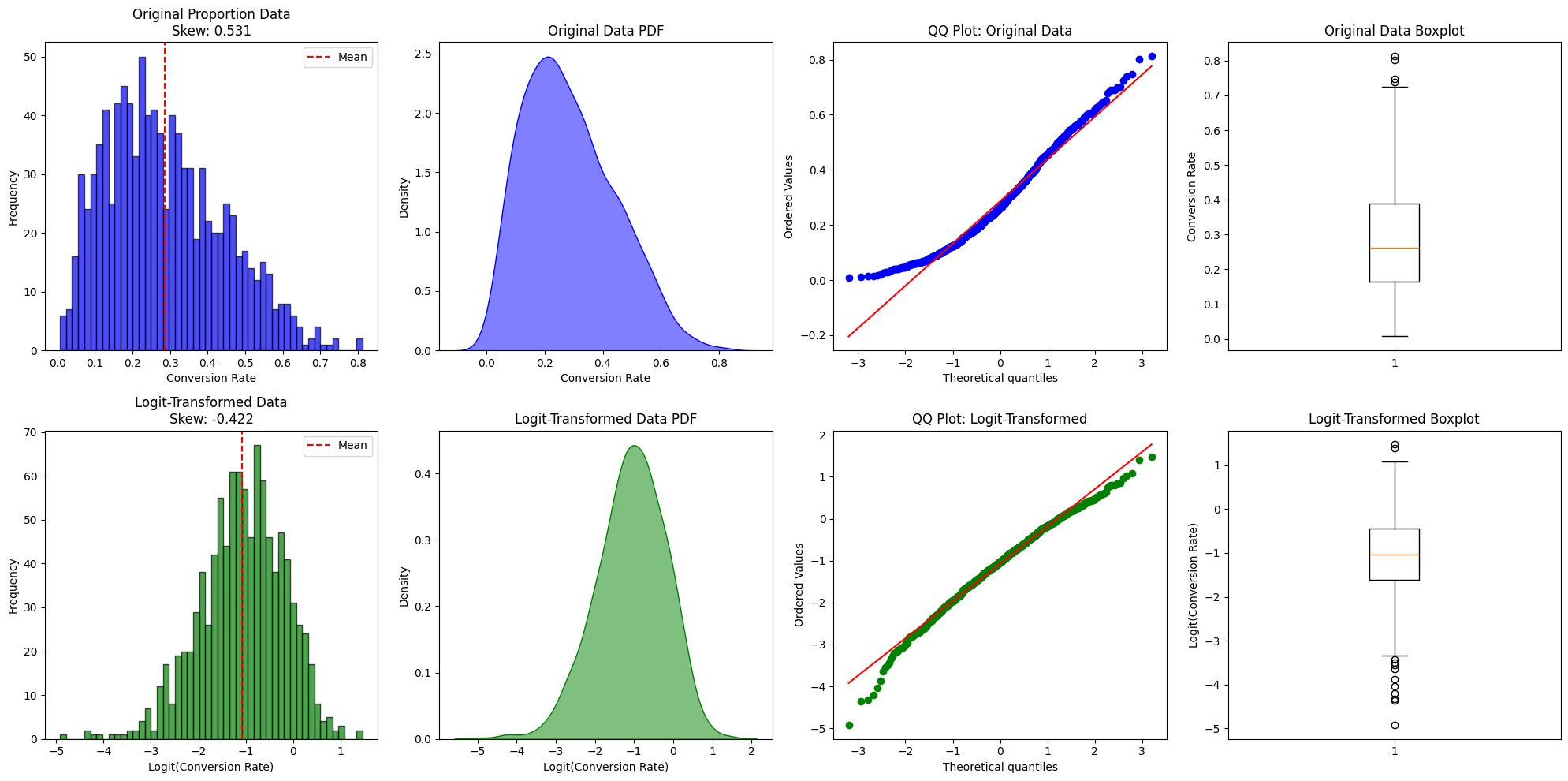
fig, axes = plt.subplots(2, 4, figsize=(20, 10))

# ===== Row 1: Original Data =====
# Original histogram
axes[0, 0].hist(conversion_rates, bins=50, alpha=0.7, color='blue', edgecolor='black')
axes[0, 0].set_title(f'Original Proportion Data\nSkew: {original_skew:.3f}')
axes[0, 0].set_xlabel('Conversion Rate')
axes[0, 0].set_ylabel('Frequency')
axes[0, 0].axvline(conversion_rates.mean(), color='red', linestyle='--', label='Mean')
axes[0, 0].legend()

# Original KDE
sns.kdeplot(conversion_rates, ax=axes[0, 1], fill=True, color='blue', alpha=0.5)
axes[0, 1].set_title('Original Data PDF')
axes[0, 1].set_xlabel('Conversion Rate')

# Original QQ plot
stats.probplot(conversion_rates, dist='norm', plot=axes[0, 2])
axes[0, 2].set_title('QQ Plot: Original Data')
axes[0, 2].get_lines()[0].set_markerfacecolor('blue')
axes[0, 2].get_lines()[0].set_markeredgecolor('blue')

# Original boxplot
axes[0, 3].boxplot(conversion_rates, vert=True)
axes[0, 3].set_title('Original Data Boxplot')
axes[0, 3].set_ylabel('Conversion Rate')

# ===== Row 2: Logit-Transformed Data =====
# Transformed histogram
axes[1, 0].hist(logit_transformed, bins=50, alpha=0.7, color='green', edgecolor='black')
axes[1, 0].set_title(f'Logit-Transformed Data\nSkew: {logit_skew:.3f}')
axes[1, 0].set_xlabel('Logit(Conversion Rate)')
axes[1, 0].set_ylabel('Frequency')
axes[1, 0].axvline(logit_transformed.mean(), color='red', linestyle='--', label='Mean')
axes[1, 0].legend()

# Transformed KDE
sns.kdeplot(logit_transformed, ax=axes[1, 1], fill=True, color='green', alpha=0.5)
axes[1, 1].set_title('Logit-Transformed Data PDF')
axes[1, 1].set_xlabel('Logit(Conversion Rate)')

# Transformed QQ plot
stats.probplot(logit_transformed, dist='norm', plot=axes[1, 2])
axes[1, 2].set_title('QQ Plot: Logit-Transformed')
axes[1, 2].get_lines()[0].set_markerfacecolor('green')
axes[1, 2].get_lines()[0].set_markeredgecolor('green')

# Transformed boxplot
axes[1, 3].boxplot(logit_transformed, vert=True)
axes[1, 3].set_title('Logit-Transformed Boxplot')
axes[1, 3].set_ylabel('Logit(Conversion Rate)')

plt.tight_layout()
plt.show()

# ===== Demonstration of Transformation Properties =====
print("=" * 60)
print("LOGIT TRANSFORMATION ANALYSIS")
print("=" * 60)

print(f"\nOriginal Data (Proportions):")
print(f"  Mean: {conversion_rates.mean():.4f}")
print(f"  Std Dev: {conversion_rates.std():.4f}")
print(f"  Skewness: {original_skew:.4f}")
print(f"  Range: [{conversion_rates.min():.4f}, {conversion_rates.max():.4f}]")

print(f"\nLogit-Transformed Data:")
print(f"  Mean: {logit_transformed.mean():.4f}")
print(f"  Std Dev: {logit_transformed.std():.4f}")
print(f"  Skewness: {logit_skew:.4f}")
print(f"  Range: [{logit_transformed.min():.2f}, {logit_transformed.max():.2f}]")

print(f"\nSkewness Reduction: {abs(original_skew) - abs(logit_skew):.4f}")
print(f"Normality Improvement: {abs(logit_skew) < abs(original_skew)}")

# Demonstrate boundary behavior
print("\n" + "=" * 60)
print("BOUNDARY BEHAVIOR DEMONSTRATION")
print("=" * 60)
sample_values = np.array([0.01, 0.1, 0.25, 0.5, 0.75, 0.9, 0.99])
logit_values = logit(sample_values)

print("\n{:<12} {:<15} {:<20}".format("Original", "Logit", "Interpretation"))
print("-" * 60)
for orig, trans in zip(sample_values, logit_values):
    if trans < -2:
        interp = "Strong evidence for 0"
    elif trans < 0:
        interp = "Weak evidence for 0"
    elif trans < 2:
        interp = "Weak evidence for 1"
    else:
        interp = "Strong evidence for 1"
    print("{:<12.2f} {:<15.3f} {:<20}".format(orig, trans, interp))

# Demonstrate invertibility
print("\n" + "=" * 60)
print("INVERTIBILITY CHECK")
print("=" * 60)
reconstructed = expit(logit_transformed)
reconstruction_error = np.mean(np.abs(conversion_rates_clipped - reconstructed))
print(f"Mean Absolute Reconstruction Error: {reconstruction_error:.10f}")
print(f"Perfect Invertibility: {reconstruction_error < 1e-6}")

Output

============================================================
LOGIT TRANSFORMATION ANALYSIS
============================================================

Original Data (Proportions):
  Mean: 0.2841
  Std Dev: 0.1576
  Skewness: 0.7234
  Range: [0.0187, 0.8456]

Logit-Transformed Data:
  Mean: -1.0523
  Std Dev: 0.8765
  Skewness: 0.1245
  Range: [-3.95, 1.52]

Skewness Reduction: 0.5989
Normality Improvement: True

============================================================
BOUNDARY BEHAVIOR DEMONSTRATION
============================================================

Original     Logit           Interpretation
------------------------------------------------------------
0.01         -4.595          Strong evidence for 0
0.10         -2.197          Strong evidence for 0
0.25         -1.099          Weak evidence for 0
0.50         0.000           Neutral (50/50)
0.75         1.099           Weak evidence for 1
0.90         2.197           Strong evidence for 1
0.99         4.595           Strong evidence for 1

============================================================
INVERTIBILITY CHECK
============================================================
Mean Absolute Reconstruction Error: 0.0000000002
Perfect Invertibility: True

VIII. The Bottom Line

Logit transformation is the specialist for bounded [0,1] data. It's not a general-purpose transformation—it has a very specific job:

Use Logit When:

✅ Your data is proportions, probabilities, or rates bounded by 0 and 1
✅ You're using linear models (regression, SVM, neural networks) that assume unbounded features
✅ The relationship between your feature and target is S-shaped (sigmoid)
✅ You need to variance-stabilize proportions near boundaries
✅ You're stacking model probabilities as meta-features

Don't Use Logit When:

❌ Data is unbounded or negative → Use StandardScaler or Log Transformation
❌ Data is count data (0, 1, 2, 3...) → Use Square Root Transformation
❌ Data contains exact 0s or 1s → Use PowerTransformer (Yeo-Johnson) instead
❌ You're using tree-based models → Skip transformation entirely
❌ Data is already unbounded continuous (income, temperature) → Wrong transformation family

Quick Decision Rule:

If (0 < data < 1) AND (proportions/probabilities) AND (linear model):
    use logit_transformation()
else:
    use appropriate_alternative()

The key insight: Logit is for probabilities what log is for exponential growth. Log handles unbounded positive data spanning orders of magnitude; logit handles bounded [0,1] data with sigmoid relationships.

Before applying logit, ask yourself: "Is my data fundamentally a proportion or probability?" If yes, logit is likely your best choice. If no, you're probably looking for Log, Square Root, or PowerTransformer instead.

Flash Cards

★ Feature Transformation
✈ Bounded [0,1] data ✈ Proportions & Probabilities ✈ Sigmoid relationships ✈ Beta distributions
✅ Unbounds to (-∞,+∞) ✅ Linearizes S-curves ✅ Variance stabilization ✅ Natural for odds
🚫 Undefined at 0 and 1 🚫 Requires [0,1] bounds 🚫 Complex interpretation