Log Transformation

Log Normalization (or Log Transformation) is a non-linear scaling technique used to compress the range of a feature that spans several orders of magnitude, especially if there are significant differences between them.

---
config:
  theme: 'base'
  layout: 'tidy-tree'
  fontSize: 5
  font-family: '"Gill Sans", sans-serif'
---
mindmap
	root(Log Normalization)
		Do Not Use When
			Negative data
			Data is already Normally distributed
			Data has any bump
			skewness was more complex than a simple exponential curve
		Use when
			Data is highly skewed
			Data is exponentially distributed

I. Features

Formula

X_{log} = \log (X + c)

Where:
- $X$ is the feature value.
- $c$ is a small constant (usually 1) to avoid log of zero.

What it does: The transformation compresses large values while expanding smaller ones, pulling heavy right tails toward a more symmetric, bell-shaped distribution. This often stabilizes variance across the range—what statisticians call reducing heteroscedasticity.

II. When Log Transformation Shines

1. Right-Skewed Distributions with Positive Values

Income data, web traffic, population counts—these naturally exhibit exponential growth patterns. Log transformation compresses large values and spreads out smaller ones, making these distributions more closer to normal and suitable for linear models.

2. Data Spanning Multiple Orders of Magnitude

When your values range from hundreds to millions (think wealth, city populations, or genomic expression levels), log transformation brings them to a comparable scale without losing relative relationships.

3. Heteroscedasticity in Regression Models

If your residuals fan out as predictions increase, log-transforming the target variable (or features) can stabilize variance, improving linear regression assumptions and prediction quality.

4. Algorithms Sensitive to Scale

Linear Regression, K-Nearest Neighbors, and Gradient Boosting Models benefit significantly. The transformation prevents features with larger absolute values from dominating distance calculations or gradient updates.

III. When to Choose Something Else

1. Zeros or Negative Values

Plain log is undefined for these cases. While you can use log1p(X) or add a constant shift, consider Yeo-Johnson transformation (via Power Transformer) instead—it handles mixed-sign data elegantly without manual intervention.

2. Already Normal or Near-Normal Data

If your distribution is already reasonably symmetric, log transformation can over-compress and introduce left skew. Stick with StandardScaler or leave the data as-is.

When data has multiple peaks or unusual shapes, log transformation won't magically create normality. Quantile Transformer is often a better choice—it maps any distribution to uniform or normal, regardless of shape.

4. Extreme Outliers Dominating the Distribution

If outliers are your main concern rather than general skewness, RobustScaler (using median and IQR) provides better protection without the non-linear warping.

5. Sparse Data

Log transformation densifies sparse matrices. If sparsity is important for computational efficiency (e.g., text features, recommendation systems), use MaxAbsScaler or StandardScaler with sparse-aware implementations.

6. Fine-Grained Differences at Lower Values Matter

The compression effect means small variations at the low end of your range get squeezed together. If these subtle differences are important for your model, reconsider the transformation.

IV. Advantages

Handles magnitude elegantly: Makes values spanning 10× to 1,000,000× comparable
Reduces skew systematically: Transforms exponential patterns into linear relationships
Stabilizes variance: Often fixes heteroscedasticity in residuals
Preserves order: Monotonic transformation maintains relative rankings
Interpretable: On log scale, multiplicative effects become additive (useful for explaining percentage changes)

V. Limitations

Domain restriction: Requires positive values; zeros need special handling
Not a universal normalizer: Won't create perfect bell curves from arbitrary distributions
Scale shift: Changes interpretation from absolute to logarithmic units
Can obscure fine-grained differences at the low end: Compression at lower values may hide important variation
Nonlinear warp: Can distort linear relationships if misapplied.
Bias near Zero: May introduce bias if the data contains values near zero.

⚠️ Log normalization doesn't "know" your specific data; it just squashes large values. If your data has a specific "bump" or if the skewness was more complex than a simple exponential curve, the log will not result in a perfect bell curve.

VI. Code Snippet

# For right-skewed data
# Add small constant to avoid log(0)
df['log_feature'] = np.log1p(df['feature'])  # log(1 + x)

# Or manually
df['log_feature'] = np.log(df['feature'] + 1)

Practical Implementation

import numpy as np
import pandas as pd
import matplotlib.pyplot as plt
import seaborn as sns
from scipy import stats
import math

# Load the dataset
housing = fetch_california_housing()
df = pd.DataFrame(housing.data, columns=housing.feature_names)

# Generate exponentially distributed sample data
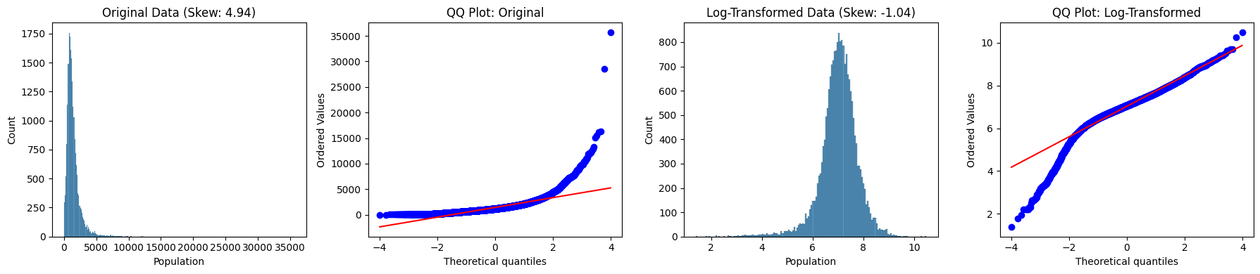
data = df['Population']
original_skew = df['Population'].skew()
log_data = np.log1p(df['Population'])  # Using log1p equivalent
log_skew = pd.Series(log_data).skew()

# Visualization
fig, axes = plt.subplots(1, 4, figsize=(18, 4))

# Original distribution
sns.histplot(data, ax=axes[0])
axes[0].set_title(f'Original Data (Skew: {original_skew:.3})')

stats.probplot(data, dist='norm', plot=axes[1])
axes[1].set_title('QQ Plot: Original')

# Log-transformed distribution
sns.histplot(log_data, ax=axes[2])
axes[2].set_title(f'Log-Transformed Data (Skew: {log_skew:.3})')

stats.probplot(log_data, dist='norm', plot=axes[3])
axes[3].set_title('QQ Plot: Log-Transformed')

plt.tight_layout()
plt.show()