StandardScaler (Z-Score Normalization)
The most common form of Standardization, where each data point is transformed by subtracting the mean and dividing by the standard deviation, resulting in a standard normal distribution.
StandardScaler transforms features such that they follow a standard normal distribution with mean = 0 and standard deviation = 1, instead of "squishing" data into a fixed box like [0, 1]. StandardScaler preserves the shape of your distribution while recentering and rescaling it.
---
config:
  theme: 'base'
  layout: 'tidy-tree'
  fontSize: 5
  font-family: '"Gill Sans", sans-serif'
---
mindmap
    root(StandardScaler)
        ✅ Use When
            Linear models (Regression, Logistic)
            Gradient-based algorithms (Neural Networks)
            Distance-based methods (KNN, SVM, K-Means)
            PCA or dimensionality reduction
            Features have different units/scales
            Near-normal distributions
        ❌ Avoid When
            Tree-based models (Random Forest, XGBoost)
            Sparse data (text, user-item matrices)
            Image data (use MinMaxScaler)
            Extreme outliers dominate
            Skewed distributions (transform first)
I. The Mechanics
Formula:
Where:
is the original feature value is the mean of the feature is the standard deviation of the feature
What it does: Each feature is transformed so that its distribution has zero mean and unit variance. This doesn't change the shape of your distribution—it just shifts and rescales it. A value that was 2 standard deviations above the mean before scaling will still be 2 standard deviations above after scaling.
II. Why StandardScaler Matters
1. The "Distance" Problem
Imagine comparing houses with two features: Square Footage (1,000–5,000) and Number of Bedrooms (1–5). Without scaling, algorithms that calculate distances (KNN, K-Means) will think a 500 sq ft difference is massively more important than a 2-bedroom difference. StandardScaler puts both features on equal footing by measuring them in standard deviations rather than raw units.
2. The "Gradient Descent" Problem
Neural Networks, Logistic Regression, and many other models use gradient descent to optimize. Without scaling:
- The optimization landscape is elongated—like a narrow canyon where the algorithm bounces back and forth
- Convergence is slow—it takes many more iterations to find the minimum
With StandardScaler, the landscape becomes spherical, allowing the optimizer to walk straight to the solution in fewer steps.
III. When StandardScaler Shines
1. Linear and Logistic Regression
These models implicitly assume features are on comparable scales. Coefficients become directly interpretable when features are standardized—a one-unit change in a standardized feature represents a one-standard-deviation change.
2. Distance-Based Algorithms
- K-Nearest Neighbors (KNN): Ensures all features contribute fairly to distance calculations
- K-Means Clustering: Prevents features with larger scales from dominating cluster formation
- Support Vector Machines (SVM): Kernel functions work best when features are on similar scales
3. Gradient-Based Optimization
Neural Networks, Gradient Boosting, and any algorithm using gradient descent converges faster and more reliably with standardized inputs.
4. Principal Component Analysis (PCA)
PCA is variance-focused. Without scaling, features with larger ranges will dominate the principal components, even if they're not actually more important. StandardScaler ensures each feature contributes based on its information content, not its scale.
5. Regularized Models (Lasso, Ridge, Elastic Net)
Regularization penalties treat all features equally. If features aren't scaled, the penalty will disproportionately affect features with smaller ranges, making the regularization ineffective.
VI. When to Choose Something Else
1. Tree-Based Models (Random Forest, XGBoost, Decision Trees)
These models are scale-invariant—they only care about the order of values, not their magnitude. Scaling adds computational overhead without any benefit.
Better approach: Skip scaling entirely for tree-based ensembles.
2. Extreme Outliers Present
StandardScaler uses mean and standard deviation, both of which are heavily influenced by outliers. A few extreme values can skew the scaling for the entire feature.
Better alternative: RobustScaler uses median and IQR (interquartile range), making it immune to outliers while still centering and scaling your data.
3. Sparse Data (Text, User-Item Matrices)
StandardScaler destroys sparsity by subtracting the mean—turning all those beautiful zeros into non-zero values. This explodes memory usage and computational cost.
Better alternatives:
- MaxAbsScaler: Preserves zeros while scaling to [-1, 1]
- No scaling: Many sparse algorithms (TF-IDF, SVD) work fine without scaling
4. Image Data (Pixel Values)
Images have a natural bounded range (0-255 for 8-bit). Neural networks typically expect inputs in [0, 1] or [-1, 1].
Better alternative: MinMaxScaler with feature_range=(0, 1) or simple division by 255.
5. Heavily Skewed Distributions
StandardScaler won't fix distributional issues—it just centers and scales whatever shape you have. If your data is exponentially distributed or has extreme right skew, standardization alone won't help.
Better approach: Apply Power Transformer (Box-Cox or Yeo-Johnson) or Log Transformation first to reduce skewness, then scale if needed.
6. New Data with Extreme Values
If test or production data contains values far outside your training range, standardized values can be extremely large (Z-scores of 100+), potentially causing numerical instability.
Better alternative: RobustScaleror careful outlier handling before scaling.
7. Interpretability Requirements
If stakeholders need to understand feature units (e.g., "dollars" or "years"), standardized values become harder to interpret.
Better approach: Document scaling parameters or use RobustScaling which is less aggressive.
V. Advantages
- Zero-centered data: Many algorithms perform better with mean-zero features
- Unit variance: Makes features directly comparable
- Preserves distribution shape: Doesn't warp your data like power transforms
- Widely supported: Default choice in most ML libraries
- Interpretable: Z-scores have universal meaning (distance from mean in standard deviations)
- Computationally efficient: Simple arithmetic operations
VI. Limitations
- Sensitive to outliers: Mean and standard deviation can be skewed by extreme values
- Destroys sparsity: Subtracting the mean creates non-zero values everywhere. It Just turns those beautiful zeros into non-zero numbers.
- Unbounded output: Unlike Min-Max, there is no set "minimum" or "maximum." Your data can go from -100 to +100 if the spread is wild.
- Assumes somewhat normal distribution: Works best when data is roughly Gaussian
- Requires storing statistics: Need to save mean and std from training data for test/production
VII. Practical Implementation
import numpy as np
import pandas as pd
import matplotlib.pyplot as plt
import seaborn as sns
from sklearn.preprocessing import StandardScaler
from sklearn.datasets import load_iris
# Load dataset
iris = load_iris(as_frame=True)
df = iris['data'][['sepal length (cm)', 'petal width (cm)']]
# Apply StandardScaler
scaler = StandardScaler()
scaled = scaler.fit_transform(df)
df_scaled = pd.DataFrame(scaled, columns=df.columns)
# Visualization
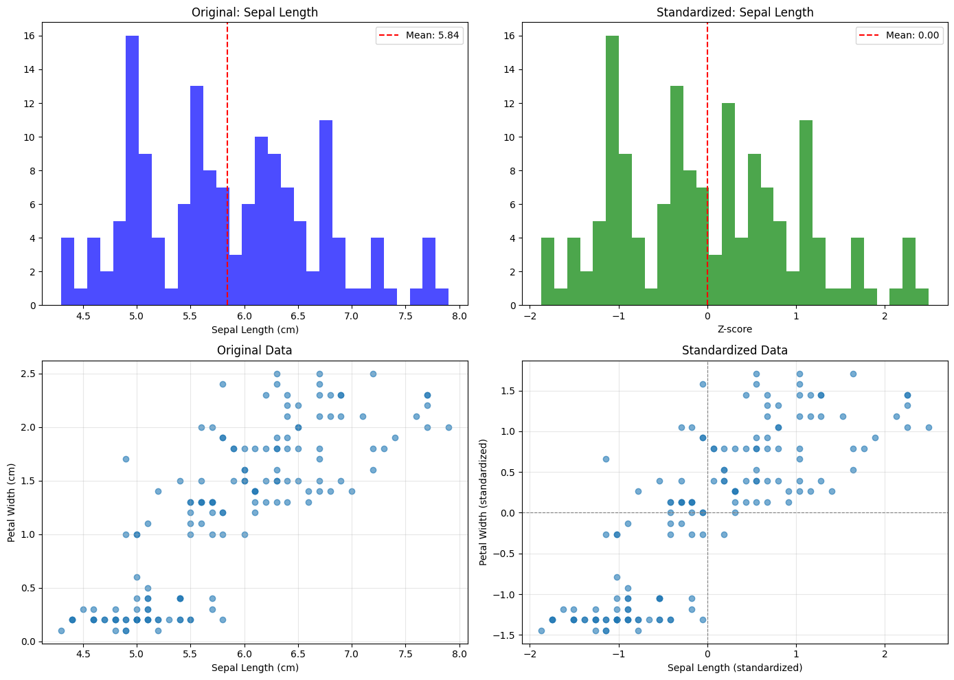
fig, axes = plt.subplots(2, 2, figsize=(14, 10))
# Original distribution
axes[0, 0].hist(df['sepal length (cm)'], bins=30, alpha=0.7, color='blue')
axes[0, 0].set_title('Original: Sepal Length')
axes[0, 0].set_xlabel('Sepal Length (cm)')
axes[0, 0].axvline(df['sepal length (cm)'].mean(), color='red', linestyle='--', label=f'Mean: {df["sepal length (cm)"].mean():.2f}')
axes[0, 0].legend()
# Scaled distribution
axes[0, 1].hist(df_scaled['sepal length (cm)'], bins=30, alpha=0.7, color='green')
axes[0, 1].set_title('Standardized: Sepal Length')
axes[0, 1].set_xlabel('Z-score')
axes[0, 1].axvline(0, color='red', linestyle='--', label='Mean: 0.00')
axes[0, 1].legend()
# Scatter plot: Original
axes[1, 0].scatter(df['sepal length (cm)'], df['petal width (cm)'], alpha=0.6)
axes[1, 0].set_xlabel('Sepal Length (cm)')
axes[1, 0].set_ylabel('Petal Width (cm)')
axes[1, 0].set_title('Original Data')
axes[1, 0].grid(True, alpha=0.3)
# Scatter plot: Scaled
axes[1, 1].scatter(df_scaled['sepal length (cm)'], df_scaled['petal width (cm)'], alpha=0.6)
axes[1, 1].set_xlabel('Sepal Length (standardized)')
axes[1, 1].set_ylabel('Petal Width (standardized)')
axes[1, 1].set_title('Standardized Data')
axes[1, 1].axhline(0, color='gray', linestyle='--', linewidth=0.8)
axes[1, 1].axvline(0, color='gray', linestyle='--', linewidth=0.8)
axes[1, 1].grid(True, alpha=0.3)
plt.tight_layout()
plt.show()
# Statistics comparison
print("Original Statistics:")
print(df.describe())
print("\nStandardized Statistics:")
print(df_scaled.describe())
Output:
Original Statistics:
       sepal length (cm)  petal width (cm)
count         150.000000        150.000000
mean            5.843333          1.199333
std             0.828066          0.762238
min             4.300000          0.100000
25%             5.100000          0.300000
50%             5.800000          1.300000
75%             6.400000          1.800000
max             7.900000          2.500000

Standardized Statistics:
       sepal length (cm)  petal width (cm)
count       1.500000e+02      1.500000e+02
mean       -4.736952e-16     -4.736952e-16
std         1.003350e+00      1.003350e+00
min        -1.870024e+00     -1.447076e+00
25%        -9.006812e-01     -1.183812e+00
50%        -5.250608e-02      1.325097e-01
75%         6.745011e-01      7.906707e-01
max         2.492019e+00      1.712096e+00
The Bottom Line
StandardScaler is the default choice for most machine learning workflows, and for good reason. It's simple, effective, and works well with the vast majority of algorithms—especially those based on gradients or distances.
However, it's not a one-size-fits-all solution. Before applying StandardScaler, ask yourself:
- Do I have outliers? → Consider RobustScaler
- Is my data sparse? → Use MaxAbsScaler or skip scaling
- Am I using tree-based models? → Skip scaling entirely
- Is my data heavily skewed? → Apply PowerTransformer first
- Do I need bounded outputs? → Use MinMaxScaler