Min-Max Scaling

Min-Max normalization (also called Min-Max scaling) is one of the most common techniques for feature scaling. It is a linear transformation technique that rescales features to a fixed range, typically [0, 1]. It's one of the most straightforward scaling methods you'll encounter, and its simplicity is both its strength and limitation.

I. The Mechanics

Formula

X_{norm} = \frac{X - X_{min}}{X_{max} - X_{min}}

Where:
$X$ is the original feature value.
$X_{min}$ is the minimum value of the feature.
$X_{max}$ is the maximum value of the feature.

What it does: The transformation linearly maps your data so that the smallest value becomes 0, the largest becomes 1, and everything else is proportionally distributed in between. This preserves the exact shape of your original distribution—just compressed into a new range.

II. When Min-Max Normalization Shines

1. Fixed Range Requirements

When your algorithm expects or performs better with bounded inputs:

Neural Networks: Activation functions like sigmoid and tanh work optimally with inputs in [0, 1] or [-1, 1]
Image Processing: Pixel values are naturally bounded (0-255), and normalization to [0, 1] is standard practice
Gradient-based optimization: Prevents features with larger ranges from dominating gradient updates

2. Distance-Based Algorithms

When your model calculates distances between data points:

K-Nearest Neighbors (KNN): Ensures all features contribute equally to distance calculations
K-Means Clustering: Prevents features with larger scales from dominating cluster formation
Support Vector Machines (SVM): Helps the kernel functions work on comparable scales

3. Preserving Zero Values in Sparse Data

When you have sparse datasets (many zeros) and those zeros carry meaning:

Text data with word counts
User-item interaction matrices in recommendation systems
Important caveat: This only works cleanly if your data is non-negative. For data with negative values where zero preservation matters, use MaxAbsScaler instead.

4. Known Feature Bounds

When you understand your data's natural boundaries:

Age (0-120 years)
Percentage values (0-100%)
Rating systems (1-5 stars)

III. When to Choose Something Else

1. Presence of Outliers

This is Min-Max normalization's Achilles heel. A single extreme value can compress the rest of your data into a tiny range, making most values indistinguishable.

Better alternative: RobustScaler uses median and interquartile range (IQR), making it robust to outliers while still scaling your data appropriately.

2. Data from Normal Distributions

If your features follow a Gaussian distribution and you're using algorithms that assume normality:

Better alternative: StandardScaler (Z-score normalization) centers data at zero with unit variance, which many statistical models expect.

3. Skewed Distributions

When your data is heavily right-skewed (exponential growth patterns, income data, web traffic):

Better alternative: Apply Log Transformation or PowerTransformer first to reduce skewness, then scale if needed. Min-Max won't fix distributional issues—it just compresses them.

4. New Data with Values Outside Training Range

If your test or production data might contain values beyond your training min/max, they'll be scaled outside [0, 1], which can break neural networks or cause unexpected behavior.

Better alternative: StandardScaler or RobustScaler handle out-of-range values more gracefully, as they don't have hard boundaries.

When your data has multiple peaks or unusual shapes

Better alternative: QuantileTransformer maps any distribution to uniform or normal, regardless of complexity.

6. Heteroscedastic Data

When variance changes across the range of your feature:

Better alternative: Consider PowerTransformer (Yeo-Johnson or Box-Cox) to stabilize variance before scaling.

VI. Advantages

Bounded output: Guarantees all values fall within [0, 1]
Uniformity: It ensures that all features have the exact same scale, preventing features with large magnitudes from dominating the model.
Preserves relationships: Linear transformation maintains relative distances and data shape
Intuitive: Easy to understand and explain
Efficient: Computationally simple and fast
Zero preservation: Maintains zeros in sparse datasets (for non-negative data)

V. Limitations

Outlier sensitivity: Extreme values severely impact scaling quality
No centering: Doesn't center data at zero, unlike StandardScaler
Range dependency: Requires knowing or estimating true min/max values
Breaks with new extremes: Fails gracefully when new data exceeds training range

VI. Practical Implementation

import numpy as np
import pandas as pd
import matplotlib.pyplot as plt
import seaborn as sns
from sklearn.datasets import load_iris
from sklearn.preprocessing import MinMaxScaler

# Load Iris dataset
iris = load_iris(as_frame=True)
df = iris['data'][['sepal length (cm)', 'petal length (cm)']]

# Apply MinMaxScaler
scaler = MinMaxScaler()
scaled = scaler.fit_transform(df)
df_scaled = pd.DataFrame(scaled, columns=df.columns)

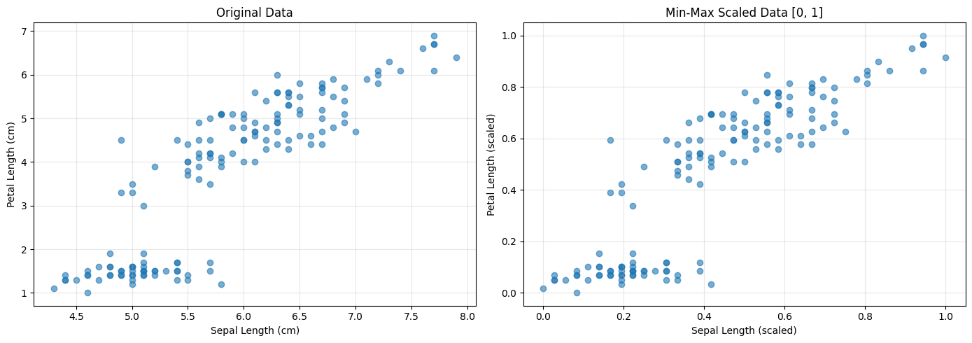
# Visualization
fig, axes = plt.subplots(1, 2, figsize=(14, 5))

# Original data
axes[0].scatter(df['sepal length (cm)'], df['petal length (cm)'], alpha=0.6)
axes[0].set_xlabel('Sepal Length (cm)')
axes[0].set_ylabel('Petal Length (cm)')
axes[0].set_title('Original Data')
axes[0].grid(True, alpha=0.3)

# Scaled data
axes[1].scatter(df_scaled['sepal length (cm)'], df_scaled['petal length (cm)'], alpha=0.6)
axes[1].set_xlabel('Sepal Length (scaled)')
axes[1].set_ylabel('Petal Length (scaled)')
axes[1].set_title('Min-Max Scaled Data [0, 1]')
axes[1].grid(True, alpha=0.3)

plt.tight_layout()
plt.show()

# Compare statistics
print("Original Data Statistics:")
print(df.describe())
print("\nScaled Data Statistics:")
print(df_scaled.describe())

Output

Original Data Statistics:
       sepal length (cm)  petal length (cm)
count         150.000000         150.000000
mean            5.843333           3.758000
std             0.828066           1.765298
min             4.300000           1.000000
25%             5.100000           1.600000
50%             5.800000           4.350000
75%             6.400000           5.100000
max             7.900000           6.900000

Scaled Data Statistics:
       sepal length (cm)  petal length (cm)
count         150.000000         150.000000
mean            0.428704           0.467458
std             0.230018           0.299203
min             0.000000           0.000000
25%             0.222222           0.101695
50%             0.416667           0.567797
75%             0.583333           0.694915
max             1.000000           1.000000