Max Abs Scaling

MaxAbsScaler is a scaling technique that divides each feature by its maximum absolute value, mapping all values to the range [-1, 1]. Its defining characteristic? It preserves zeros—making it invaluable for sparse datasets where most values are zero.

---
config:
  theme: 'base'
  layout: 'tidy-tree'
  fontSize: 5
  font-family: '"Gill Sans", sans-serif'
---
mindmap
    root(MaxAbsScaler)
        ✅ Use When
            Sparse data with many zeros
            Mixed positive and negative values
            Zero preservation is critical
            Centered data preferred
            SVM or sparse algorithms
        ❌ Avoid When
            Extreme outliers present
            Zero-mean required
            Normal distribution needed
            Dense data without zeros

I. The Mechanics

Formula:

• Where $max(|X|)$ is the absolute maximum value of the feature.

What it does: Each feature is independently scaled by dividing every value by the largest absolute value in that feature. This guarantees the scaled range falls within [-1, 1], while preserving the sign and zero values perfectly.

Key insight: Unlike MinMaxScaler or StandardScaler, MaxAbsScaler doesn't shift data—it only scales. This is what keeps your zeros exactly at zero, maintaining sparsity.

II. When Max Abs Scaling Shines

1. Sparse Data (The Primary Use Case)

When your dataset is dominated by zeros—text data with word counts, user-item interaction matrices, or any high-dimensional sparse representation:

• Preserves computational efficiency of sparse matrices
• Doesn't artificially create non-zero values where they don't exist
• Keeps memory footprint minimal

2. Mixed Sign Data Where Zero is Meaningful

When your features naturally contain both positive and negative values, and zero represents a true neutral point:

• Financial data (profit/loss, account balances)
• Temperature differences from a baseline
• Sentiment scores ranging from negative to positive

3. Support Vector Machines (SVM) with Sparse Data

SVMs with linear kernels perform well when data is centered, and MaxAbsScaler maintains that property while preserving sparsity—a perfect match.

4. Data Already Centered at Zero

If your features are already centered (mean ≈ 0) and you just need to control the scale, MaxAbsScaler provides simple, efficient scaling without unnecessary shifting.

III. When to Choose Something Else

1. Presence of Extreme Outliers

This is MaxAbsScaler's critical weakness. A single extreme value compresses the rest of your data into a tiny, unusable range.
Example: If your feature has values [1, 2, 3, 4, 1000], everything except 1000 gets squished to nearly zero: [0.001, 0.002, 0.003, 0.004, 1.0].

Better alternative: RobustScaler uses median and IQR, effectively ignoring outliers while still scaling your data appropriately.

2. Dense Data (Few or No Zeros)

When your data doesn't have meaningful zeros or sparsity to preserve, MaxAbsScaler offers no advantage over simpler alternatives.

Better alternatives:

• MinMaxScaler: When you need bounded [0, 1] output
• StandardScaler: When you need zero-mean, unit-variance scaling

3. Algorithms Requiring Zero-Mean Data

Neural networks, PCA, and many statistical models perform better when features are centered at zero with comparable variance.

Better alternative: StandardScaler explicitly centers data at zero and scales to unit variance—exactly what these algorithms expect.

4. Skewed or Non-Normal Distributions

MaxAbsScaler won't fix distributional issues—it just scales the existing distribution.

Better alternative: Apply PowerTransformer (Yeo-Johnson) or QuantileTransformer first to address skewness, then scale if needed.

5. Text Data with TF-IDF

While text data is sparse, TF-IDF already handles appropriate weighting and scaling for most NLP tasks.

Better approach: Use TF-IDF directly without additional scaling, unless you're combining text features with other numeric features.

6. Feature Ranges Matter for Interpretation

If you need to maintain original units or interpretable ranges (e.g., for reporting to stakeholders), MaxAbsScaler's [-1, 1] transformation obscures the original scale.

Better alternative: Use RobustScaler or even leave data unscaled if the model permits.

VI. Advantages

• Preserves sparsity: Keeps zeros exactly at zero—critical for sparse matrices
• Maintains signs: Positive values stay positive, negative stay negative
• No centering: Doesn't shift data, only scales
• Computationally efficient: Single division per value
• Handles mixed-sign data: Works seamlessly with both positive and negative values
• Bounded output: Guarantees [-1, 1] range

V. Limitations

• Outlier sensitivity: Extreme values severely compress the rest of your data
• No centering guarantee: Doesn't produce zero-mean data
• Limited use case: Primarily beneficial only for sparse data
• Fixed range: Strict [-1, 1] bounds may not suit all algorithms
• Doesn't fix distribution: Won't address skewness or non-normality

VI. Practical Implementation

import numpy as np
import pandas as pd
import matplotlib.pyplot as plt
import seaborn as sns
from sklearn.preprocessing import MaxAbsScaler
from scipy.sparse import csr_matrix

# Example 1: Sparse data (the ideal use case)
sparse_data = {
    'Feature1': [-45, -10, 0, 10, 20], 
    'Feature2': [0, 50, 0, 75, 100],
    'Feature3': [0, 0, 0, 0, 200]  # Highly sparse
}
df_sparse = pd.DataFrame(sparse_data)

# Apply MaxAbsScaler
scaler = MaxAbsScaler()
scaled_sparse = scaler.fit_transform(df_sparse)
df_scaled = pd.DataFrame(scaled_sparse, columns=df_sparse.columns)

print("Original Sparse Data:")
print(df_sparse)
print("\nScaled Data (preserves zeros):")
print(df_scaled)
print("\nMax absolute values used for scaling:")
print(scaler.max_abs_)

# Example 2: Demonstrating outlier sensitivity
outlier_data = {
    'Normal_Range': [1, 2, 3, 4, 5],
    'With_Outlier': [1, 2, 3, 4, 1000]
}
df_outlier = pd.DataFrame(outlier_data)

scaler_outlier = MaxAbsScaler()
scaled_outlier = scaler_outlier.fit_transform(df_outlier)
df_scaled_outlier = pd.DataFrame(scaled_outlier, columns=df_outlier.columns)

print("\n--- Outlier Sensitivity Example ---")
print("Original:")
print(df_outlier)
print("\nScaled (notice compression):")
print(df_scaled_outlier)

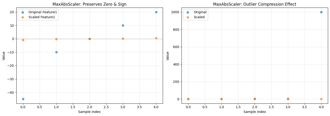
# Visualization
fig, axes = plt.subplots(1, 2, figsize=(14, 5))

# Sparse data comparison
x = range(len(df_sparse))
axes[0].scatter(x, df_sparse['Feature1'], label='Original Feature1', alpha=0.7)
axes[0].scatter(x, df_scaled['Feature1'], label='Scaled Feature1', alpha=0.7)
axes[0].axhline(y=0, color='gray', linestyle='--', linewidth=0.8)
axes[0].set_xlabel('Sample Index')
axes[0].set_ylabel('Value')
axes[0].set_title('MaxAbsScaler: Preserves Zero & Sign')
axes[0].legend()
axes[0].grid(True, alpha=0.3)

# Outlier effect
axes[1].scatter(x, df_outlier['With_Outlier'], label='Original', alpha=0.7)
axes[1].scatter(x, df_scaled_outlier['With_Outlier'], label='Scaled', alpha=0.7)
axes[1].set_xlabel('Sample Index')
axes[1].set_ylabel('Value')
axes[1].set_title('MaxAbsScaler: Outlier Compression Effect')
axes[1].legend()
axes[1].grid(True, alpha=0.3)

plt.tight_layout()
plt.show()

Output:

Original Sparse Data:
   Feature1  Feature2  Feature3
0       -45         0         0
1       -10        50         0
2         0         0         0
3        10        75         0
4        20       100       200

Scaled Data (preserves zeros):
   Feature1  Feature2  Feature3
0 -1.000000      0.00       0.0
1 -0.222222      0.50       0.0
2  0.000000      0.00       0.0
3  0.222222      0.75       0.0
4  0.444444      1.00       1.0

Max absolute values used for scaling:
[ 45. 100. 200.]

--- Outlier Sensitivity Example ---
Original:
   Normal_Range  With_Outlier
0             1             1
1             2             2
2             3             3
3             4             4
4             5          1000

Scaled (notice compression):
   Normal_Range  With_Outlier
0           0.2         0.001
1           0.4         0.002
2           0.6         0.003
3           0.8         0.004
4           1.0         1.000