I. Feature Transformation & Scaling: A Step-by-Step Guide
Feature transformation and scaling are not random operations—they require systematic analysis of your data's characteristics to choose the right technique. This guide provides a clear, decision-driven approach to transform and scale features effectively.
flowchart LR
    Start([Start:
Raw
Dataset]) --> Step1[Step 1:
Understand
Your Data]
    Step1 --> Step2[Step 2:
Check
Distribution]
    Step2 --> Step3[Step 3:
Identify
Problems]
    Step3 --> Step4[Step 4:
Choose
Transformation]
    Step4 --> Step5[Step 5:
Apply
Transformation]
    Step5 --> Step6[Step 6:
Validate
Results]
    Step6 --> Decision{Is Distribution
Acceptable?}
    Decision -- No --> Step4
    Decision -- Yes --> Step7[Step 7:
Apply
Scaling]
    Step7 --> End([Ready
for
Modeling])

    style Start fill:#e3f2fd,stroke:#1976d2,stroke-width:3px,color:#0d47a1
    style End fill:#c8e6c9,stroke:#388e3c,stroke-width:3px,color:#1b5e20
    style Decision fill:#fff3e0,stroke:#f57c00,stroke-width:2px,color:#e65100
    style Step1 fill:#e1f5fe,stroke:#0288d1,stroke-width:2px
    style Step2 fill:#e1f5fe,stroke:#0288d1,stroke-width:2px
    style Step3 fill:#e1f5fe,stroke:#0288d1,stroke-width:2px
    style Step4 fill:#fff9c4,stroke:#fbc02d,stroke-width:2px
    style Step5 fill:#fff9c4,stroke:#fbc02d,stroke-width:2px
    style Step6 fill:#f3e5f5,stroke:#8e24aa,stroke-width:2px
    style Step7 fill:#c8e6c9,stroke:#388e3c,stroke-width:2px
Step 1: Understand Your Data
★ Purpose: Know what you're working with before making any changes.
★ Actions:
-
Load your dataset and examine basic statistics
-
Identify feature types (numerical vs. categorical)
-
Check for missing values and outliers
-
Understand the domain context (e.g., prices, ages, probabilities)
# Load and examine data
df = pd.read_csv('your_data.csv')

# Basic statistics
print(df.describe())
print(df.info())

# Check missing values
print(df.isnull().sum())
★ Outcome: A clear understanding of your data's structure, range, and potential issues.
Step 2: Check Data Distribution
★ Purpose: Data distribution represents how values of a dataset are spread across a range. It shows how your data is distributed to identify patterns, skewness, presence of outliers and anomalies.
★ Common Data Distribution
- Normal distribution (bell-shaped)
- Right-skewed (long tail on right)
- Left-skewed (long tail on left)
- Bimodal (two peaks)
- Presence of outliers
- Uniform (flat distribution)
- Sparse Data
- Range (Positive, Negative, zeros)
★ Options for Visualization
- Histogram with KDE (Kernel Density Estimate)
# Single feature sns.histplot(df['feature_name'], kde=True, bins=30) - Multiple Features at Once
# Grid of histograms df.hist(figsize=(15, 10), bins=30) - Box Plot / Violin Plot (for outliers)
# Single feature sns.boxplot(data=df, x='feature_name') - QQ Plot (Quantile-Quantile)
from scipy import stats
stats.probplot(df['feature_name'], dist="norm", plot=plt)
Step 3: Identify Problems
I. Purpose
Diagnose specific issues that require transformation.
II. Problem Checklist
| Problem | How to Detect | Impact on ML Models |
|---|---|---|
| Skewness | df['feature'].skew() (>1 or <-1 is significant) |
Biases linear models, affects distance-based algorithms |
| Different Scales | Features range from 0-1 while others 0-10,000 | Dominates gradient descent, distance calculations |
| Non-Linearity | Scatter plot shows curve, not straight line | Poor fit for linear models |
| Non-Gaussian Distribution | Histogram doesn't look bell-shaped | Violates assumptions of many algorithms |
| Outliers | Box plots show extreme points | Skews scaling, affects model performance |
| Bounded Data | Values confined to [0,1] or percentages | May need specific scaling techniques |
III. Code to Check
★ Check skewness for all numerical features
skewness = df.select_dtypes(include=[np.number]).skew()
print("Skewness:\n", skewness)
★ Check for non-linearity (correlation matrix)
print(df.corr())
★ Visualize relationships
sns.pairplot(df)
plt.show()
Step 4: Choose Transformation
I. Purpose
Select the appropriate transformation based on identified problems.
II. Decision Matrix
★ Distinguishing when to Use Each Transformation
This table clarifies the specific distinguishing cases for choosing the right transformation:
| Problem Identified | Transformation Options | When to Use Each |
|---|---|---|
| Right-Skewed Data | 1. LogTransformation 2. Square Root Transformation 3. Box-Cox |
Log: Exponential growth patterns (income, prices) Sqrt: Moderate skew Box-Cox: Automatic optimal transformation |
| Left-Skewed Data | 1. Reflect + Log 2. Square Transformation 3. Yeo-Johnson |
Reflect: Mirror data first Square: Mild left-skew Yeo-Johnson: Handles negatives |
| Non-Gaussian (Any Shape) | 1. Box-Cox 2. Yeo-Johnson 3. Quantile Transformer |
Box-Cox: Positive values only Yeo-Johnson: With negatives Quantile: Force specific distribution |
| Non-Linear Relationships | 1. Polynomial Transformation 2. LogTransformation 3. Exponential |
Polynomial: Captures curves Log: Exponential relationships Exp: Inverse of log |
| Probabilities/Proportions | 1. Logit Transformation | Converting probabilities to unbounded scale |
| Bounded Data (0-1) | 1. Logit Transformation 2. Probit |
Both expand bounded values |
| Extreme Outliers | 1. Winsorization 2. Clipping 3. RobustScaler |
Cap extreme values before other transformations |
★ Evaluating Each Transformation
As alternate method, We can iterate each transformer and see if it can be applied to our feature column(s)
ᯓ ᯓ ✈︎ Refer Feature Transformation Summary for detailed view
Step 5: Apply Transformation
I. Code Snippet References
Execute the chosen transformation and create new features.
★ LogTransformation
★ Box-Cox Transformation
★ Yeo-Johnson Transformation
★ Polynomial Transformation
★ LogitTransformation
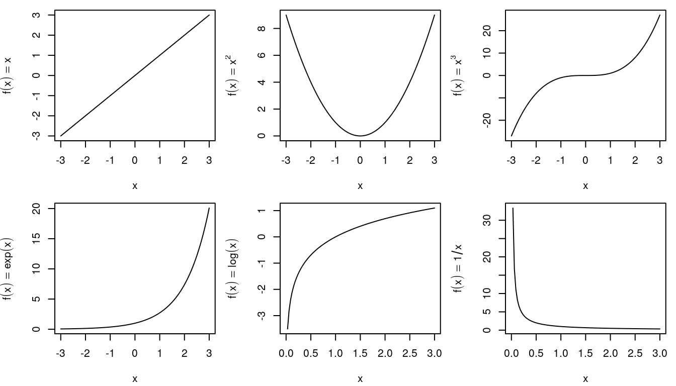
★ Square Transformation (x²)
★ Square Root Transformation (√x)
★ Reciprocal Transformation (1/x)
★ QuantileTransformer
Step 6: Validate Results
I. Purpose
Verify that transformation improved the distribution.
★ Visual Comparison
fig, axes = plt.subplots(1, 2, figsize=(12, 4))

# Before transformation
sns.histplot(df['original_feature'], kde=True, ax=axes[0])
axes[0].set_title('Before Transformation')

# After transformation
sns.histplot(df['transformed_feature'], kde=True, ax=axes[1])
axes[1].set_title('After Transformation')

plt.tight_layout()
plt.show()
★ Statistical Tests
from scipy.stats import shapiro, normaltest

# Shapiro-Wilk test for normality (p > 0.05 = normal)
stat_before, p_before = shapiro(df['original_feature'])
stat_after, p_after = shapiro(df['transformed_feature'])

print(f"Before: p-value = {p_before:.4f}")
print(f"After: p-value = {p_after:.4f}")

# Check skewness improvement
print(f"\nSkewness Before: {df['original_feature'].skew():.2f}")
print(f"Skewness After: {df['transformed_feature'].skew():.2f}")
★ QQ Plot Comparison
from scipy import stats

fig, axes = plt.subplots(1, 2, figsize=(12, 4))

stats.probplot(df['original_feature'], dist="norm", plot=axes[0])
axes[0].set_title('QQ Plot: Before')

stats.probplot(df['transformed_feature'], dist="norm", plot=axes[1])
axes[1].set_title('QQ Plot: After')

plt.tight_layout()
plt.show()
★ Success Criteria:
- ✅ Skewness reduced (closer to 0)
- ✅ Distribution looks more Gaussian
- ✅ QQ plot points closer to diagonal line
- ✅ Statistical test p-value improved
- ✅ Outliers reduced or managed
Step 7: Apply Scaling
I. Purpose
After transformation, scale features so they contribute equally to model training.
II. Scaling Decision Matrix:
| Data Characteristics | Recommended Scaler |
|---|---|
| Gaussian Distribution No Outliers |
StandardScaler |
| Bounded Range Needed (e.g., Neural Networks) |
MinMaxScaler |
| Significant Outliers Present | RobustScaler |
| Sparse Data (many zeros) | MaxAbsScaler |
| Extreme Outliers | Quantile Transformer |
| Non-Gaussian After Transform | Power Transformer |