Line Plot

Purpose

Visualize trends over time or continuous sequences. Essential for time series analysis and trend identification.

Analysis Type

Bivariate (typically time vs. value)

What to Look For

1. Trends

• Upward: Increasing over time
• Downward: Decreasing over time
• Flat: No trend
• Cyclical: Repeating patterns

2. Seasonality

• Regular repeating patterns
• Daily, weekly, monthly, yearly cycles
• Important for time series forecasting

3. Volatility

• Amount of variation in the data
• High volatility = large fluctuations
• Low volatility = stable values

4. Outliers/Anomalies

• Sudden spikes or drops
• Unusual patterns
• May indicate data errors or significant events

5. Multiple Series

• Compare trends across different groups
• Identify divergence or convergence
• Look for correlations between series

6. Change Points

• Sudden changes in level or trend
• May indicate regime changes or interventions

Code Example

# Example: Line plots using seaborn's flights dataset
import seaborn as sns
import matplotlib.pyplot as plt

# Load sample dataset
flights = sns.load_dataset('flights')

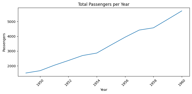
# Basic line plot: Passengers over time (by year)
plt.figure(figsize=(8, 4))
yearly = flights.groupby('year')['passengers'].sum().reset_index()
plt.plot(yearly['year'], yearly['passengers'])
plt.title("Total Passengers per Year")
plt.xlabel("Year")
plt.ylabel("Passengers")
plt.xticks(rotation=45)
plt.tight_layout()
plt.show()

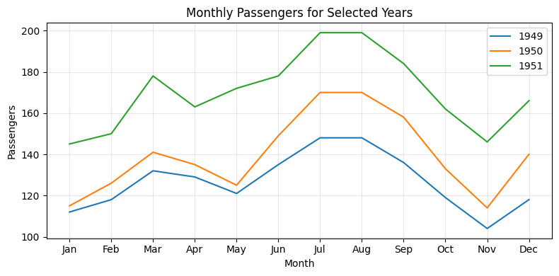
# Multiple lines: Passengers per month for a few years
sample_years = [1949, 1950, 1951]
months = flights['month'].unique()
plt.figure(figsize=(8, 4))
for year in sample_years:
    data = flights[flights['year'] == year]
    plt.plot(months, data['passengers'], label=str(year))

plt.title("Monthly Passengers for Selected Years")
plt.xlabel("Month")
plt.ylabel("Passengers")
plt.legend()
plt.grid(True, alpha=0.3)
plt.tight_layout()
plt.show()

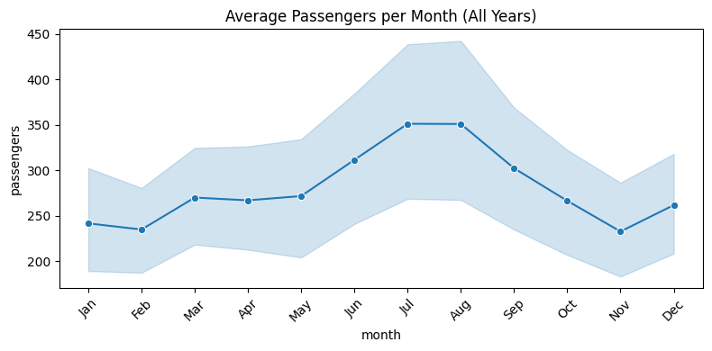
# Seaborn lineplot with confidence interval (trend by month across years)
plt.figure(figsize=(8, 4))
# Convert month to categorical for correct order
flights['month'] = pd.Categorical(flights['month'], categories=months, ordered=True)
sns.lineplot(x='month', y='passengers', data=flights, estimator='mean', marker='o')
plt.title("Average Passengers per Month (All Years)")
plt.xticks(rotation=45)
plt.tight_layout()
plt.show()