Pearson Correlation

🛡️ Pearson Correlation

Unlocking Features with Pearson Correlation

In univariate feature selection, we look at one feature at a time against the target variable. The Pearson test checks: “Does this feature have a linear relationship with the target?”

The Pearson Correlation Test is like your quick “chemistry check” in feature selection. It tells you which features sing in harmony with the target, but it’s not the whole story. Think of it like auditioning singers for a band. Each singer (feature) tries a solo with the lead guitarist (target). If they harmonize well (high correlation), they’re shortlisted; if they’re off-key, they’re out.

What is Pearson Correlation?

Pearson correlation measures how strongly two variables move together.

If one goes up and the other goes up too → positive correlation (like height and weight).
If one goes up and the other goes down → negative correlation (like hours of Netflix bingeing and exam grades).
If there’s no pattern → no correlation (like shoe size and salary).

\begin{aligned} r & = \frac{\sum (x_{i} - \bar{x}) (y_{i} - \bar{y})}{\sqrt{\sum (x_{i} - \bar{x})^{2} (y_{i} - \bar{y})^{2}}} \end{aligned}

where:

$x_{i}$ , $y_{i}$ are the data points
$\bar{x}$ , $\bar{y}$ are their means
$r$ ranges from -1 to 1
- $r$ = 1 → perfect positive sync
- $r$ = -1 → perfect negative sync
- $r$ = 0 → no sync at all

Code Snippet

1. Numeric Features with Regression Target


import pandas as pd  
import numpy as np  
from scipy.stats import pearsonr  
  
# Example dataset  
df = pd.DataFrame({  
    'study_hours': [1, 2, 3, 4, 5, 6],  
    'exam_score': [35, 50, 65, 70, 80, 90]  
})  
  
# Pearson correlation  
corr, p_value = pearsonr(df['study_hours'], df['exam_score'])  
print("Correlation:", corr, "P-value:", p_value)

Output

Correlation: 0.98   P-value: 0.0003

2. Categorical Features with Numeric Target

Pearson correlation is not directly suitable for categorical data.
But you can transform categories into numbers (via one-hot encoding or label encoding) and then test.

⚠️ Be cautious: encoding categories imposes an artificial order.
For pure categorical features, Chi-square is a better choice.

🧭 Using 'Pearson Correlation' for Multivariate Feature Selection in Regression Problems

1: Pearson is inherently univariate

By definition, Pearson correlation works pairwise — it compares one feature at a time with the target variable.

That’s why it’s primarily used for univariate feature selection in regression:

You compute r(feature, target) for every feature.
Then select the top-k features with the strongest absolute correlation.

But what if your data has many interrelated features? That’s where the multivariate part comes in.

2: Extending Pearson to a Multivariate Setting

When dealing with multiple features, Pearson’s correlation can help in two complementary ways

🔹 1. Feature-to-Target Correlation (Relevance)

You still compute the correlation between each feature and the target — to measure how useful a feature is.

import pandas as pd  
from sklearn.datasets import fetch_california_housing  
  
data = fetch_california_housing(as_frame=True)  
  
# Separate the features and target variable  
X = data.data  
target = data.target_names[0]  
X[target] = data.target  
  
corr_with_target = X.corr()[target].drop(target).sort_values(ascending=False)  
print(corr_with_target)

output

MedInc            0.688075  
AveRooms      0.151948  
HouseAge       0.105623  
AveOccup       -0.023737  
Population       -0.024650  
Longitude        -0.045967  
AveBedrms     -0.046701  
Latitude           -0.144160  
Name: MedHouseVal, dtype: float64

This helps identify which features are most linearly predictive of the target.

🔹 2. Feature-to-Feature Correlation (Redundancy)

Then, you compute the correlation between features themselves — to detect multicollinearity (refer at the bottom for details).

Why? Because in a multivariate regression model, highly correlated features provide redundant information and can confuse the model.

import seaborn as sns  
import matplotlib.pyplot as plt  
  
corr_matrix = X.drop(data.target_names[0], axis=1).corr()  
  
plt.figure(figsize=(8,6))  
sns.heatmap(corr_matrix, annot=True, cmap='coolwarm')  
plt.title("Feature-to-Feature Correlation Matrix")  
plt.show()

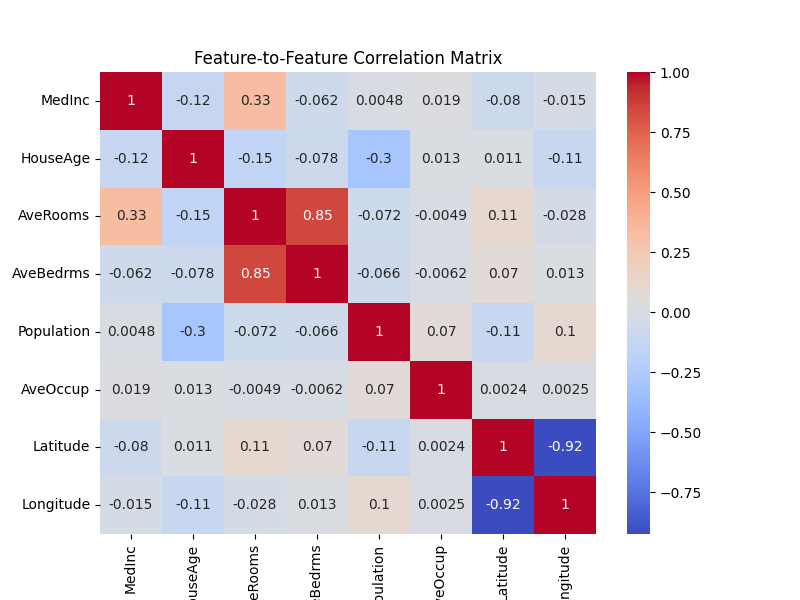
If two features have correlation |r| > 0.9, you might want to keep only one of them.

🎯 The Multivariate Strategy

You can combine these two ideas into a filter-based multivariate feature selection process:

Compute correlation of all features with target (relevance).
Remove features that are highly correlated with each other (redundancy).
Select top features that are both relevant and not redundant.

✅ Best for:

Regression problems with linear relationships
Early-stage exploratory feature screening
Numeric features (continuous data)
Models like Linear Regression, Lasso, Ridge, ElasticNet

👍 Pros

Simple and fast — easy to compute, even on large datasets.
Interpretable — everyone understands “strong” vs “weak” correlation.
Good for numeric regression targets — naturally fits continuous outcomes.

👎 Cons

Only linear relationships — it misses non-linear patterns (e.g., quadratic or exponential).
Sensitive to outliers — one extreme value can distort correlation.
Not ideal for categorical features — needs encoding, which may mislead. For Ordinal or categorical features, use Spearman, Kendall, or Mutual Information instead and Situations with severe multicollinearity use PCA or VIF-based filtering

🚧 Caution

Correlation ≠ Causation — Just because two things move together doesn’t mean one causes the other. Ice cream sales and drowning deaths both rise in summer, but one doesn’t cause the other.
Check assumptions — Works best with continuous, normally distributed data.
Watch out for multicollinearity — Features highly correlated with each other can confuse models.

What is Multicollinearity?

Multicollinearity happens when two or more input features (independent variables) are highly correlated with each other, rather than just with the target.

Why is it a problem?

Confuses the model
In regression, the model tries to assign a weight (coefficient) to each feature. If two features tell the same story (e.g., “height in cm” and “height in inches”), the model struggles to decide which one deserves the credit. The result: unstable or misleading coefficients.
Inflated variance
Estimates of coefficients swing wildly depending on tiny changes in the data. That makes the model less reliable.
Interpretability loss
If your goal is to explain which features matter most, multicollinearity makes it murky.

How to Detect It?

Correlation matrix → check if features are highly correlated (|r| > 0.9).
Variance Inflation Factor (VIF) → a statistical measure where high values (>10) suggest multicollinearity.

How to Fix It

Drop one of the correlated features (keep the one that’s more variance and is more interpretable).
Combine them (e.g., average, or use dimensionality reduction like PCA).
Regularization (Lasso/Ridge regression can reduce the effect).

🧠 Pearson is your first filter, not the final judge.

Common Questions

How Correlation-Based Selection Works in both Feature Selection and Feature Elimination:?
- ✅ Feature Selection:
  - If you retain the best set of independent features (e.g., using a threshold to keep only important features), it's a feature selection method.
- ✅ Feature Elimination:
  - If you remove highly correlated features to avoid redundancy, it's a feature elimination method.
```
import pandas as pd
import numpy as np

corr_matrix = pd.DataFrame(X).corr().abs()
upper = corr_matrix.where(np.triu(np.ones(corr_matrix.shape), k=1).astype(bool))
to_drop = [column for column in upper.columns if any(upper[column] > 0.9)]
X_selected = pd.DataFrame(X).drop(columns=to_drop)
```