Bias, Variance, Overfitting & Underfitting
At the heart of every machine learning project lies a fundamental challenge: creating a model that not only learns from the data it's given but also generalizes to make accurate predictions on new, unseen data. A model's ability to do this is constantly pulled between two opposing forces: Bias and Variance.
Think of it like a student preparing for an exam.
- A student who only memorizes the answers to practice questions might ace the practice test but will likely fail the final exam, which has slightly different questions. This is overfitting.
- A student who only learns a few high-level concepts but doesn't study the details might perform poorly on both the practice test and the final exam. This is underfitting.
The goal is to be the student who understands the underlying concepts deeply enough to solve both familiar and new problems. In machine learning, this sweet spot is achieved by balancing bias and variance.
This document will break down these critical concepts:
- Bias: The simplifying assumptions a model makes.
- Variance: The model's sensitivity to the training data.
- Underfitting: The problem of a model being too simple (high bias).
- Overfitting: The problem of a model being too complex (high variance).
- The Bias-Variance Tradeoff: The central balancing act of model building.
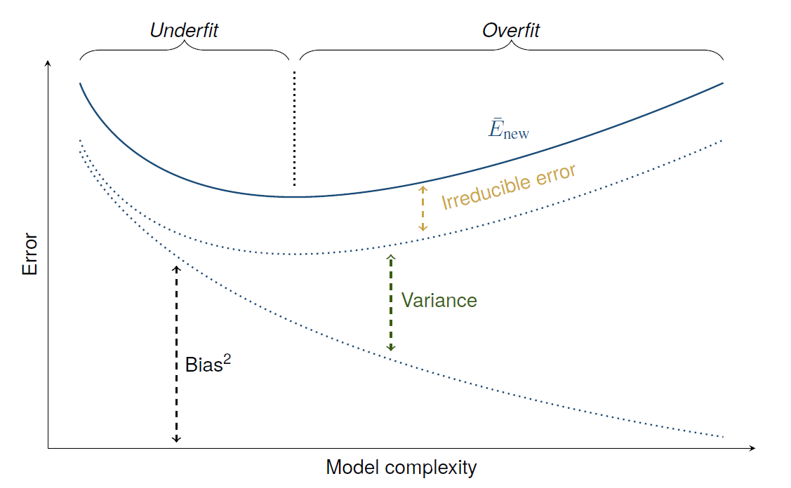
I. The Two Types of Model Error
When we evaluate a model, the errors it makes can be broken down into two categories:
1. Irreducible Error (The "Unknowable")
This is the error that we can never get rid of, no matter how sophisticated our model is. It represents the inherent randomness and complexity of the real world that our data can't capture.
Sources of Irreducible Error
- Unobserved Variables: There may be influential factors that affect the outcome but are not included in the model because they were not measured or are unknown. For example, a model predicting house prices can't account for the buyer's sentimental attachment to a neighborhood.
- Data Noise: Data can contain random noise due to inaccuracies in measurement, data entry mistakes, or other unpredictable factors.
- Stochastic Processes: The underlying process generating the data might have an inherent randomness that cannot be captured by the model. For example, human behavior can be inherently unpredictable.
- Approximation Errors: Even the best models are only approximations of real-world phenomena, which are often too complex to be captured perfectly by any model.
This error sets a theoretical "best possible" performance for any model on our data. Our job is to minimize the other kind of error.
2. Reducible Error (The Part We Can Control)
Reducible errors are the types of errors in a machine learning model that can be reduced or minimized through various techniques, such as better modeling, improved data quality, or more sophisticated algorithms. These errors arise from the limitations and imperfections of the model and the training process.
Sources of Reducible Errors
- Bias
- Variance
- Bias²: Error caused by incorrect assumptions in the model.
- Variance: Error caused by sensitivity to training data.
- Irreducible Error: Random noise in the data that cannot be eliminated.
II. Bias and Underfitting
What is Bias?
Bias refers to the inability of a machine learning model to capture the true relationship between the data variables. It is caused by the erroneous assumptions that are inherent to the learning algorithm.
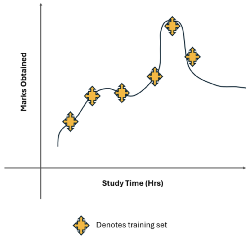
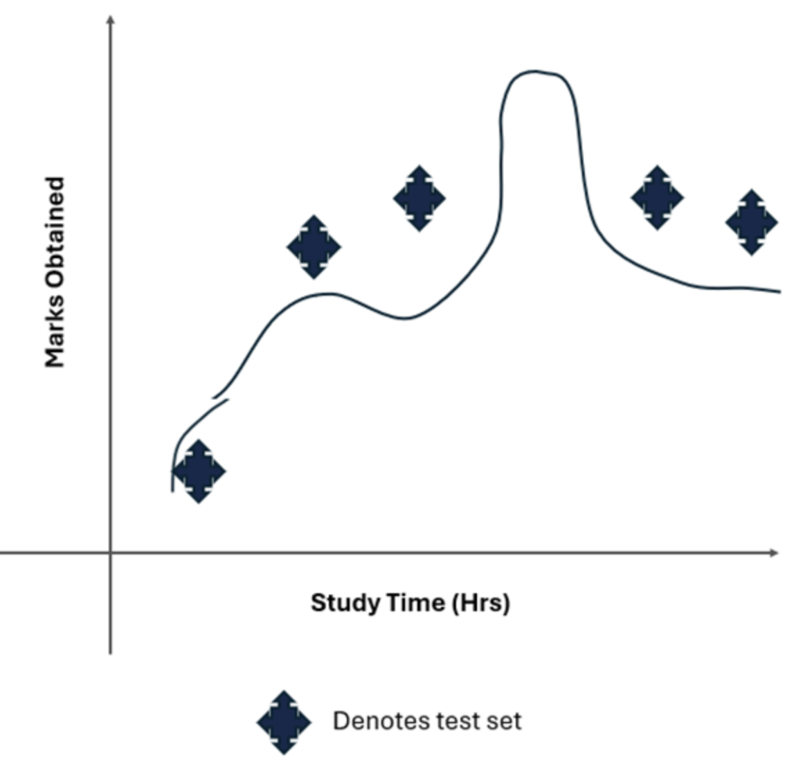
Example: Consider a scenario in which you want to predict students' marks based on the number of hours they study. A simple linear regression model is used to make this prediction. The model assumes a straight-line relationship between study time and marks.
- Model Assumption:
- Actual Relationship: The relationship between study time and marks might be more complex. For example, the relationship might be quadratic or logarithmic because after a certain number of study hours, additional hours may contribute less to marks, or too much study could lead to fatigue and lower performance.
- Assumed Relationship: If a linear regression model is used to fit a straight line through the data points, it assumes a linear relationship
- Missed Pattern: It cannot capture the actual curving pattern of the data. This gives rise to systematic errors where the predictions from the linear model will deviate from the actual marks. In other words, the linear model oversimplifies the relationship, leading to underfitting.
Types of Bias
- Low Bias:
- The model captures patterns well and is closer to the true values.
- A model incorporates fewer assumptions about the target function. (e.g., A decision tree can split data in complex ways).
- The model is flexible enough to follow the data "signal" tightly. While this reduces training error, it can lead to high variance if the model is too sensitive to noise (overfitting).
- High Bias:
- The model oversimplifies, misses patterns and underfits the data.
- A high bias model typically includes more assumptions about the target function or end result.
- If the true relationship is a complex curve, a high-bias linear model fails to learn the training data patterns effectively, resulting in low accuracy on both training and testing data. It implies the model is too rigid, such as a straight line attempting to fit a curved dataset.
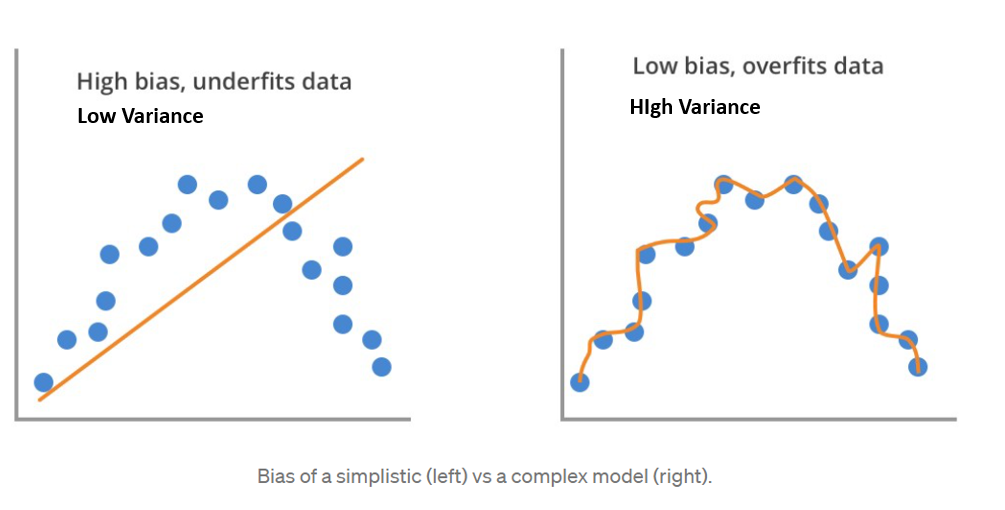
A high-bias linear model fails to capture the true, curved relationship in the data.
The consequence of High Bias ➛ Underfitting
When a model has high bias, it leads directly to underfitting. An underfit model overly simplistic and cannot capture the underlying structure of the data.
- How to Diagnose Underfitting:
The tell-tale sign of underfitting is poor performance on both the training data and the test data. The model isn't just failing on new data; it couldn't even learn the original data properly.- High Training Error: The model makes significant errors on the data it was trained on.
- High Test Error: The model also performs poorly on new, unseen data.
III. Variance and Overfitting
★ What is Variance?
Variance is the error from a model's excessive sensitivity to small fluctuations in the training data. A model with high variance is unstable. If you were to train it on a slightly different subset of your data, you would get a completely different model.
- Low Variance: A model's results are consistent across different training sets. (e.g., Linear regression is stable).
- High Variance: A model changes significantly with small changes in the training data. (e.g., A high-degree polynomial or a very deep decision tree).
High-variance models are so flexible that they learn not only the underlying signal in the data but also the noise. They essentially "memorize" the training set.
A high-variance model (like the green line) wiggles and turns to fit every single point, including the noise.
★ Overfitting: The Consequence of High Variance
When a model has high variance, it leads directly to overfitting. An overfit model is too complex and has tailored itself perfectly to the training data.
Example
- A complex model fits the training data almost perfectly, resulting in near-zero error.
- On the test data, the same complex model performs poorly because it's trying to apply the "noise" it learned to new data, where that noise doesn't exist.
- In logistic regression, very large coefficients often indicate that the model is trying too hard to fit the training data, capturing noise along with the signal. This is a sign of overfitting, where the model becomes too complex and performs well on the training data but poorly on unseen data.
How to Diagnose Overfitting?
The classic sign of overfitting is a huge gap between the model's performance on training data versus test data.
- Low Training Error: The model makes very few errors on the data it was trained on. It seems perfect.
- High Test Error: When given new data, the model performs poorly because it memorized noise instead of learning the general pattern.
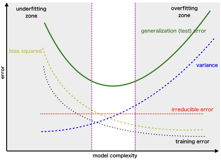
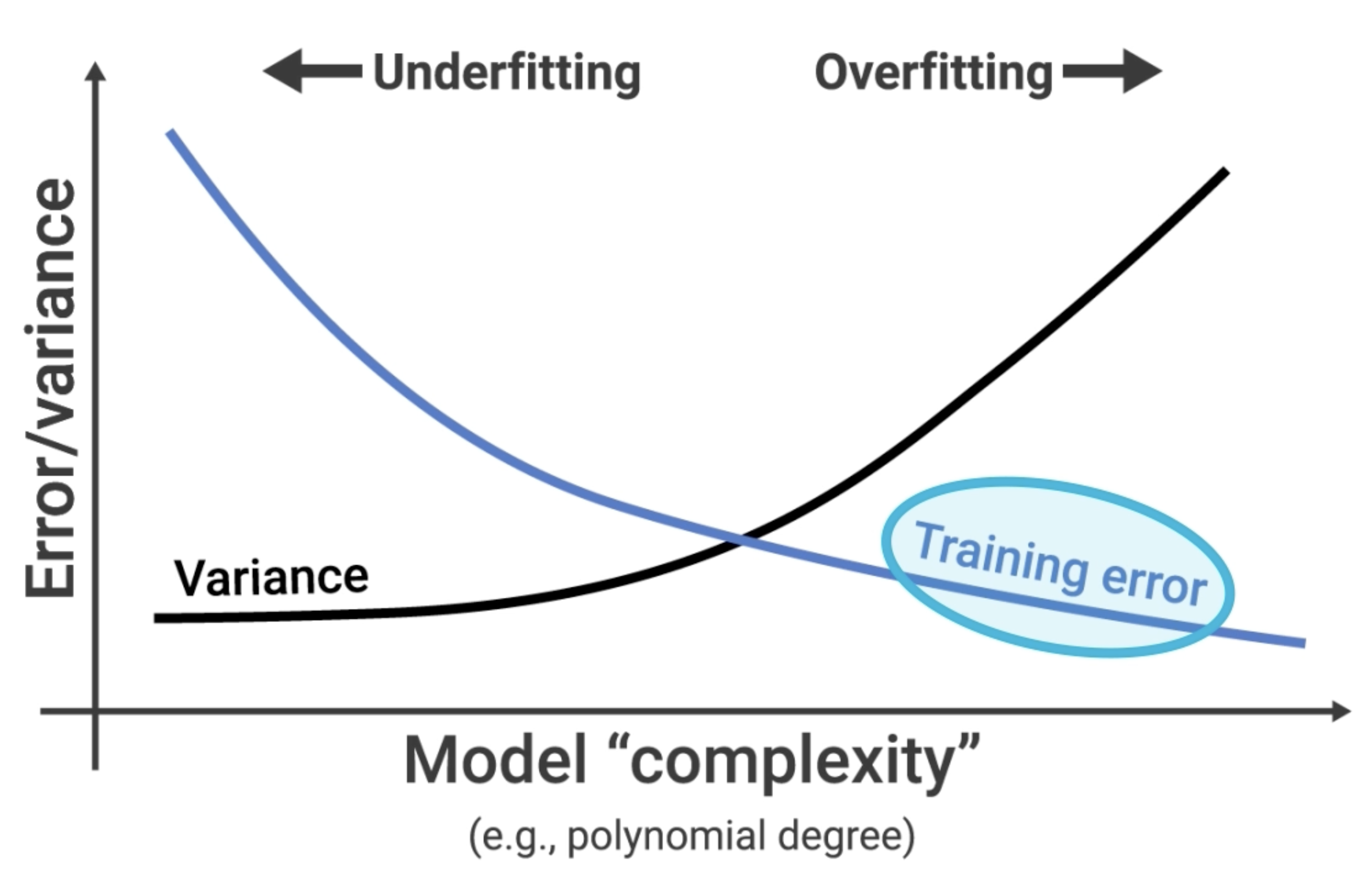
IV. The Bias-Variance Tradeoff
This brings us to the most important concept: the Bias-Variance Tradeoff. It's the central challenge of building a good model.
- Simple Models (like Linear Regression) are high-bias and low-variance. They are stable but can't capture complex patterns. They are prone to underfitting.
- Complex Models (like a deep Decision Tree) are low-bias and high-variance. They are flexible enough to capture complex patterns but are unstable and can easily learn noise. They are prone to overfitting.
The relationship is a zero-sum game. As you decrease bias (by making the model more complex), you inevitably increase variance. As you decrease variance (by making the model simpler), you inevitably increase bias.
The Goal: Our goal is not to find a model with zero bias and zero variance. That's impossible. Our goal is to find the "sweet spot"—the level of model complexity that minimizes the total error (the sum of bias-squared and variance). This is the model that generalizes best to new data.
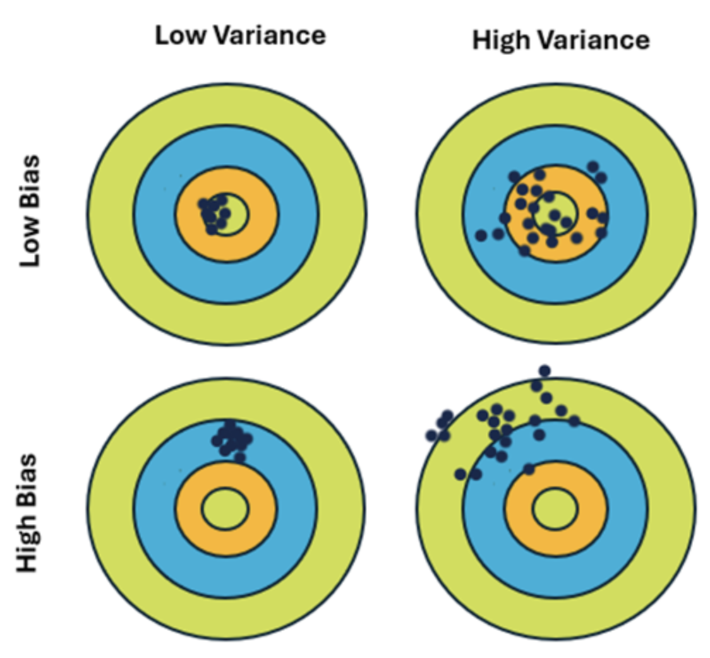
★ The Bullseye Target ★
ᯓ ✈︎ Strongly recommend to read The Bullseye Target example, which is covered separately
★ Diagnosing the Problem
Here’s a simple guide to diagnosing whether your model suffers from high bias or high variance:
| Model State | Training Error | Test Error | Diagnosis |
|---|---|---|---|
| Underfitting | High | High | High Bias. The model is too simple. |
| Overfitting | Low | High | High Variance. The model is too complex and memorized the training set. |
| 🎯 Good Fit | Low | Low | Low Bias & Low Variance. The model is just right and generalizes well. |
| Avoid | High | Even Higher | High Bias & High Variance. The model is just bad. It's simple enough that it can't learn the data, but it's also unstable. This is rare but can happen with poor feature choices. |
V. How to Fix Bias and Variance Problems
Once you've diagnosed your model's issue, you can apply targeted strategies to fix it.
How to Fix High Bias (Underfitting)
If your model is too simple, you need to increase its complexity.
1. Use a More Complex Model:
Switch from a simple model like linear regression to a more powerful one like a gradient boosting machine (XGBoost), a random forest, or a neural network.
2. Add More Features (Feature Engineering):
The model might be missing the right information.
- Create Polynomial Features: Adding squared or cubed terms (
) or interaction terms ( ) can help a linear model capture curves. - Add Domain-Specific Features: Use your knowledge of the problem to create new features that might be relevant.
3. Decrease Regularization:
Regularization techniques (like L1 and L2) are designed to reduce complexity. If your model is already too simple, you should reduce the strength of the regularization hyperparameter (e.g., decrease C in SVMs/Logistic Regression, decrease alpha in Ridge/Lasso).
How to Fix High Variance (Overfitting)
If your model is too complex and has memorized the training data, you need to reduce its complexity or give it more data to generalize from.
1. Get More Training Data:
This is often the most effective solution. With more data, the model has a harder time memorizing noise and is forced to learn the true underlying pattern.
2. Reduce the Number of Features (Feature Selection):
A model with too many features can easily overfit.
- Use feature selection algorithms (e.g., based on feature importance from a tree model, or using statistical tests) to keep only the most predictive features.
3. Increase Regularization:
Apply or increase the strength of regularization.
- L1 Regularization (Lasso): Can shrink some feature coefficients to exactly zero, effectively performing feature selection.
- L2 Regularization (Ridge): Shrinks all coefficients, preventing any single feature from having too much influence.
- Dropout (for Neural Networks): Randomly deactivates neurons during training, forcing the network to learn redundant representations.
4. Simplify the Model:
- For Decision Trees:
- Reduce the maximum depth of the tree (
max_depth) or - increase the minimum number of samples required to make a split (
min_samples_split). This is called "pruning."
- Reduce the maximum depth of the tree (
- For Neural Networks: Use a smaller network with fewer layers or fewer neurons per layer.
5. Use Cross-validation
While not a direct fix, using a robust cross-validation strategy ensures that your evaluation of the model's performance is accurate and that you aren't being fooled by a lucky train-test split.
6. Ensembling Methods
Techniques like Bagging (e.g., Random Forest) and Boosting (e.g., Gradient Boosting) can be very effective.
- Bagging helps reduce variance by averaging the predictions of multiple models trained on different subsets of the data.
VI. Generalization and Cross-Validation
The Tools for Building Robust Models
★ What is Generalization?
Generalization is the ultimate goal of a machine learning model. It refers to a model's ability to perform well on new, unseen data after having been trained on a finite dataset.
- A model that generalizes well has found the true underlying pattern in the data. Its performance is consistent between the training set and the test set.
- A model that generalizes poorly has either underfit (and didn't learn the pattern) or overfit (and learned the noise).
All the techniques for fixing bias and variance are ultimately in service of improving generalization.
★ Using Validation to Find the Sweet Spot
So how do we find the model with the best generalization—the one at the bottom of the total error curve? We can't use the test set, because if we tune our model based on the test set, we are "leaking" information from it, and it no longer provides an unbiased estimate of performance on unseen data.
This is where a validation set comes in.
The standard workflow is to split your data into three parts:
- Training Set: Used to train the model (i.e., fit the parameters).
- Validation Set (or Development Set): Used to tune the model's hyperparameters (like the degree of a polynomial, the
kin KNN, or the strength of regularization). You choose the hyperparameter settings that give you the best performance on the validation set. - Test Set: Used only once, at the very end, to get a final, unbiased evaluation of how well your chosen model generalizes.
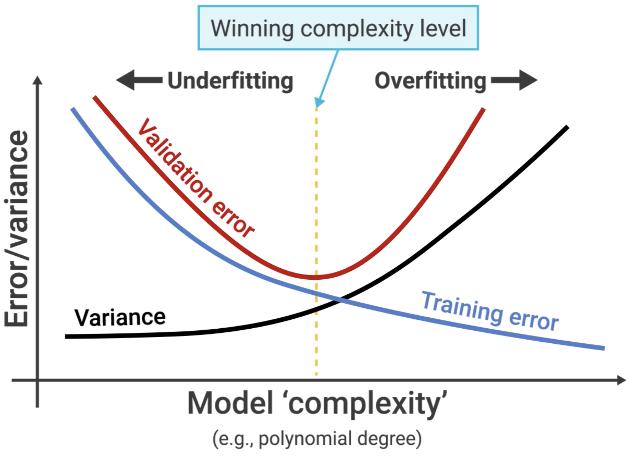
The validation error is our proxy for the test error. We tune our model's complexity to find the minimum point on the validation curve.
★ The Problem with a Simple Validation Set
A simple train/validation split has a problem: the performance can be highly dependent on which specific data points happened to end up in the validation set. If you got a "lucky" or "unlucky" split, your evaluation might be misleading.
★ K-Fold Cross-Validation: A More Robust Approach
K-Fold Cross-Validation is a more robust and widely used technique to solve this problem.
How it works:
- Split your data into K equal-sized "folds" (e.g., K=5 or K=10).
- Perform K rounds of training and validation:
- In each round, use one fold as the validation set and the remaining K-1 folds as the training set.
- Average the validation scores from all K rounds. This average score is your final performance estimate.
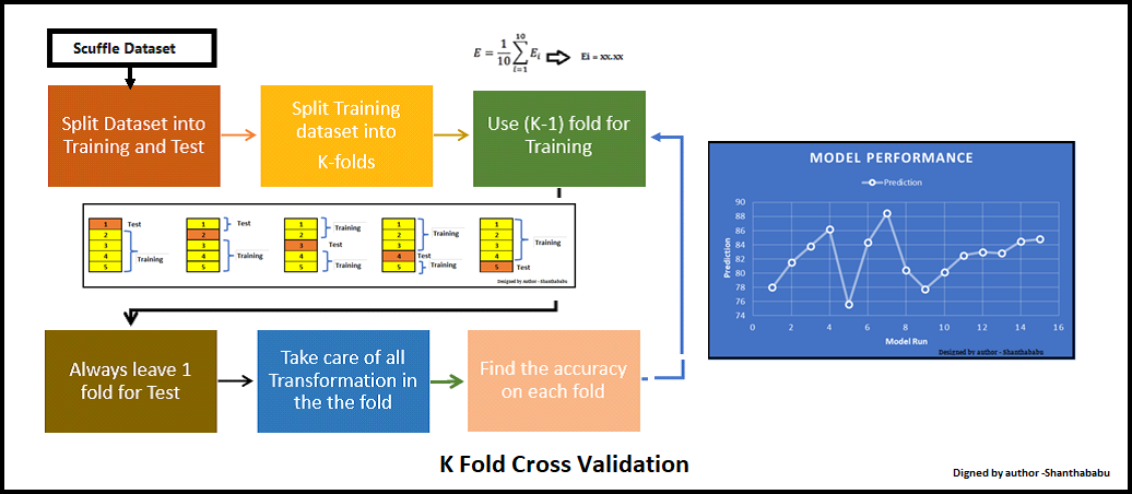
Advantages of K-Fold Cross-Validation:
- More Reliable: The performance estimate is much more stable and less dependent on a single random split.
- Efficient Data Usage: Every data point gets to be in a validation set exactly once and in a training set K-1 times.
By using cross-validation to tune your hyperparameters, you can be much more confident that you are finding the true "sweet spot" of the bias-variance tradeoff and building a model that will generalize well to the real world.